PROFESSIONAL TECHNICAL AND SCIENTIFIC PAPERS

 

Real-time gypsum quality estimation in an industrial calciner: A neural network-based approach

 

 

M. Jacobs^*; R-D. Taylor; F.H. Conradie; A.F. van der Merwe

School of Chemical and Minerals Engineering, North-West University, Potchefstroom, South Africa

Correspondence

 

 

---

SYNOPSIS

Total bound moisture (TBM) is a typical quality indicator of industrial-grade gypsum. This gypsum is comprised of three distinct phases, namely anhydrite, dihydrate, and hemihydrate, of which only the latter is of much industrial use. TBM analysis is a lengthy laboratory procedure, and an artificial neural network (ANN) TBM inference measurement is proposed as a fast and online alternative. An ANN inference model for gypsum TBM based on plant data was developed. The inputs to the network were primarily focused on the plant's calciner, and different network topologies, data divisions, and transfer functions were investigated. Furthermore, the applicability of the TBM value as a quality indicator was investigated based on a gypsum phase analysis. A strong correlation between TBM and the gypsum hemihydrate and anhydrite content was found, validating the plant target TBM of 5.8% as a quality indicator. A network topology consisting of one hidden layer with logarithmic-sigmoid (logsig) and pure linear (purelin) transfer functions showed the best performance (R > 90%).

Keywords: gypsum, artificial neural network, Levenberg-Marquardt algorithm.

---

 

 

Introduction

Calcium sulphate and its phases

Calcium sulphate hemihydrate (CaSO₄½H₂O), commonly known as bassanite or Plaster of Paris, is widely used in various industries, ranging from construction to medicine and even the arts. Pure gypsum (calcium sulphate dihydrate) is found in nature as a compact rock. Therefore, to obtain the valuable bassanite, the gypsum is calcined according to Equation [1] (Dantas et al., 2007).

The dehydration reaction of gypsum to bassanite occurs at 100-120°C and is complete at 160°C (Dantas et al, 2007). The bassanite occurs in two forms: α-hemihydrate and β-hemihydrate (Singh and Middendorf, 2007). α-Hemihydrate is formed in wet process units such as autoclaves, and β-hemihydrate is formed in predominantly dry conditions, such as in calciners (Singh and Middendorf, 2007).

Further dehydration of bassanite leads to calcium sulphate anhydrite according to Equation [2] (Dantas et al., 2007).

Similarly to bassanite, three types of anhydrite are formed during thermal dehydration, namely III-anhydrite (AIII), II-anhydrite (AII), and I-anhydrite (AI) (Li and Zhang, 2021). Anhydrite III is the first dehydration phase that forms from bassanite, followed by an unusable form of gypsum anhydrite, namely anhydrite II, and lastly, anhydrite I upon further heating. However, the latter form is unstable below 1180°C (Cave, 2000; Rajković et al, 2009).

AIII is metastable at ambient conditions and rehydrates in the presence of water or water vapour (Cave, 2000). When a large amount of soluble anhydrite (AIII) is blended into cement, it can result in a substantial expansion of the concrete and adversely impact the cement's strength (Tzouvalas, Dermatas, and Tsimas, 2004). Furthermore, insoluble gypsum anhydrite (AII) affects the hydration reaction rate and amount of unusable material in the gypsum calciner product (Christensen et al., 2008).

Gypsum in industry

Natural gypsum contains approximately 3% equilibrium moisture and 20 mass% crystal moisture (Dantas et al., 2007). The partially dehydrated form of gypsum, calcium sulphate hemihydrate (CaSO₄½H₂O), is the desired product for use in the construction, ceramic, and medical industries (Singh and Middendorf, 2007). The hydration of calcium sulphate hemihydrate (bassanite) is an exothermic reaction, given by Equation [3] (Singh and Middendorf, 2007). During hydration (in paste form), the plaster sets, which develops the strength of the material (Singh and Middendorf, 2007).

This research study investigated synthetic gypsum produced from the phosphoric acid fertilizer manufacturing process (MechChem Africa, 2019; Jordan and van Vuuren, 2022). This phosphogypsum is formed according to the reaction given by Equation [4] (Rajković et al., 2009):

From Equation [4], it is clear that a substantial amount of phosphogypsum is produced with the phosphoric acid. In fact, according to Li and Zhang (2021), approximately 5 t of phosphogypsum is produced per ton of phosphoric acid, resulting in the generation of 280 Mt of phosphogypsum waste per year worldwide.

Phosphogypsum must be calcined to deactivate impurities before being used as a building material, as these impurities impact the strength and settling times of the gypsum product (Li and Zhang, 2021; Tzouvalas, Dermatas, and Tsimas, 2004). According to Singh and Garg (cited by Tzouvalas, Dermatas, and Tsimas, 2004; Li and Zhang, 2021), impurities are deactivated by coatings of insoluble calcium pyrosulphate at elevated temperatures. Similarly, Liu et al., (cited by Li and Zhang, 2021) found that soluble phosphorus was converted to insoluble calcium pyrophosphate through calcination at 800°C for 1 hour. Additionally, fluoride and phosphorus pentoxide can be removed at 700°C, with phosphatic impurities also being removed at 800°C. According to Saadaoui et al., (2017), the radioactive components in phosphogypsum can be considered negligible.

Calcination also produces gypsum hemihydrate by driving off crystal moisture (Koper et al., 2020). In the case of gypsum, the dihydrate phosphogypsum is calcined, and a mixture of calcium sulphate dihydrate, hemihydrate, and anhydrite is obtained (Koper et al., 2020). However, the amount of calcium sulphate anhydrite (especially the insoluble form) should be minimized (Christensen et al., 2008). This is because insoluble calcium sulphate anhydrite adds to the impurities in the gypsum, adversely affecting the quality. Furthermore, a high calcium sulphate anhydrite content i results in a significant increase in the heat of hydration of the mixture (Tydlitat, Medved, and Cerny, 2012). This would affect the properties of the gypsum, such as setting time, resulting in flash setting, which impacts the quality and strength of the gypsum (Tydlitat, Medved, I. and Cerny, 2012, p. 62; Tzouvalas, Dermatas, and Tsimas, 2004, p. 2113).

Therefore, quality control of the gypsum product from an industrial plant is of utmost importance to ensure the desired specifications are met. The total bound moisture (TBM) is often used as a quality control parameter. A simple method to determine TBM is thermogravimetric analysis (TGA), where the sample is dried and mass loss indicates the moisture in the original sample. Gürsel et al., (2021) investigated acoustic emission (AE) technology to determine the gypsum and anhydrite contents online. Seufert et al., (2009) used X-ray diffraction (XRD) analysis to determine the phase composition of dehydrated gypsum. However, Dantas et al., (2007, p. 692) found that XRD cannot be used to distinguish between the hemihydrate and anhydrite phases due to the superposition of the peaks. This was confirmed by Seufert et al., (2009, p. 940), who concluded that 'high quality and high resolution' XRD data is required for successful identification.

Artificial neural networks

An artificial neural network (ANN) receives inputs that are multiplied by a weight (Krenker, Bester, and Kos, 2011). A transfer function in the body then transforms the summation of the weighted inputs and bias to produce an output. However, this output is initially meaningless as the weight and bias coefficients are random. Therefore, the network is trained using feed-forward or recurrent (feedback) learning algorithms, which adjust the weights and biases to a point where the network functions independently to make decisions predictively (Abraham, 2005). The key to understanding neural network training lies in first reviewing the basics of neural network transfer functions, which connect the input, hidden, and output layers.

The transfer functions are typically log-sigmoid, hyperbolic tangent, sine or cosine, and linear functions. The sigmoid function is widely used and performs well for classification problems involving learning about average behaviour (Zhang, Patuwo, and Hu, 1998). The logarithmic-sigmoid (log-sigmoid) function is mathematically described by Equation [5] and produces an output between 0 and 1.

The hyperbolic tangent sigmoid function is typically used for forecasting problems where the network learns about the deviations from the average (Zhang, Patuwo, and Hu, 1998). This function, which is given by Equation [6], produces an output between -1 and 1.

Alternatively, the sine or cosine and linear functions can be used as transfer functions. The sine and cosine function outputs also vary between 1 and -1, whereas that of the linear function is unbounded. However, the output values generated by these functions would have to be normalized (Zhang, Patuwo, and Hu, 1998).

Learning algorithms

The backpropagation learning algorithm (also known as the steepest decent algorithm) is one of the most powerful ANN learning algorithms (Caocci et al., 2011, p. 223; Yu and Wilamowski, 2011). With enough hidden layers, the backpropagation learning algorithm can approximate any nonlinear function (Abraham, 2005, p. 904). This method converges asymptotically, resulting in slow convergence, especially near the solution (Yu and Wilamowski, 2011; Zhang, Patuwo, and Hu, 1998). Furthermore, according to Zhang, Patuwo, and Hu (1998), the backpropagation method is inefficient, lacks robustness, and is very sensitive to the learning rate (a). Small α-values result in very slow learning, whereas large a-values may result in oscillations (Zhang, Patuwo, and Hu, 1998). Another training algorithm that minimizes a quadratic error function is Newton's method (Abraham, 2005). This method exhibits fast convergence but performs well only for almost linear systems, which is not the case in ANNs (Wilamowski, 2011).

The Levenberg-Marquardt algorithm is a combination of the steepest descent (backpropagation) and the Gauss-Newton algorithms. When the solution is far from the desired one, the algorithm behaves like the steepest descent algorithm - slow but sure to converge (Lourakis, 2005; Yu and Wilamowski, 2011). Similarly, when the current solution is close to the desired one, the algorithm behaves like the Gauss-Newton algorithm (Lourakis, 2005; Yu and Wilamowski, 2011). The Levenberg-Marquardt algorithm is regarded as one of the most efficient training algorithms and has been found to apply to small and medium-sized problems (Brezak et al, 2012; Yu and Wilamowski, 2011). According to Alwosheel, van Cranenburgh, and Chorus (2018) the sizes of the training data-sets are typically between 10 and 100 times the number of weights in the neural network.

Topology

The topology of a neural network is situational-dependent, meaning that one size does not fit all. The following list summarizes important characteristics to consider when designing an ANN:

► The training data should consist of all the characteristics of the problem. The more complex the problem is, the more data is required (Abraham, 2005, p. 904).

► Noise or randomness in the data will aid the creation of a robust and reliable ANN (May, Dandy, and Maier, 2011, p. 19).

► One hidden layer is sufficient for many practical problems (Heaton, 2008, p. 158)

► The network is usually trained for a specific number of epochs or until the error decreases below a specified threshold (Abraham, 2005, p. 904). However, care must be taken not to overtrain the network (Wilamowski, 2011, p. 16). This will result in a network that is too adapted to the training examples and will be unable to classify samples outside of the training set (Wilamowski, 2011, p. 16). Overtraining can be avoided by (Azadi and Karimi-Jashni, 2016, p. 19):

► Dividing the available data-set into training, validation, and test sets (Azadi and Karimi-Jashni, 2016, p. 19).

► The training set is used to train the model and is fed through the network during each epoch (Baheti, 2022).

► The validation set is used to validate the performance of the model during the training process (Baheti, 2022). The validation set is used to determine the stopping point - this will prevent overtraining the network (Azadi and Karimi-Jashni, 2016, p. 19). The model is validated after each epoch (Baheti, 2022).

► The test set is used after the training is completed to confirm the results (Baheti, 2022).

► The number of neurons in the hidden layer affects the performance of the network (Abraham, 2005, p. 904). A large number of hidden neurons will ensure proper training and forecasting; however, overtraining may occur (Sheela and Deepa, 2013, p. 1). Contrarily, too few hidden neurons will result in poor training and large errors (Sheela andDeepa, 2013, p. 1). Although many guidelines exist on the appropriate number of hidden neurons, it ultimately comes down to trial and error (Heaton, 2008, p. 159)

► The chosen initial weights are crucial for proper convergence; however, no recommendations exist in this regard (Abraham, 2005, p. 905). A trial-and-error approach should be followed to improve the results obtained.

► The learning rate influences the step size by which the weight is updated. A too-fast learning rate may result in overstepping the local minimum. This could result in oscillations and slow convergence. Similarly, a too-slow learning rate will result in a large number of oscillations, also resulting in slow convergence (Abraham, 2005, p. 905).

Problem statement

Laboratory analysis of the quality parameter (total bound moisture -TBM) associated with gypsum calcination into a hemihydrate form is time-consuming, thus prohibiting proper quality control of such equipment.

Motivation

The residence time in f the calcination plant in question is very short (less than half an hour). However, conventional quality analyses, such as thermogravimetric and XRD, take significantly longer to complete. Furthermore, the laboratory methods already established on the plant were used for analyses. Therefore, this study investigates the possibility of implementing a soft sensor, which can be developed using ANNs. Using this soft sensor, the quality of the gypsum product can be estimated in real-time with the current plant conditions.

 

Theory

Model software

The neural network toolbox of Matlab^TM R2021a (using Windows 11 Pro on a machine running Intel^® Core™ i5-8350U CPU @ 1.70 GHz, 8.0 GB RAM 64-bit operating system), specifically the nftool function, was initially used to obtain access to the ANN environment. Subsequently, the graphical interface of the nftool function was used to generate the relevant Matlab^TM code. This code could then be adapted for different topologies, transfer functions, and training data divisions.

Model procedure

Data division

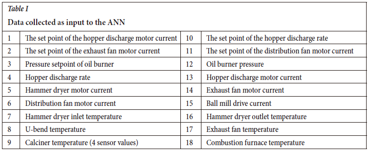
The training data comprises inputs and an output, where the inputs are made up of the collected data described in Table I and the output is the experimentally obtained TBM. The input dataset (comprising 813 data-sets) is divided into the training and simulation sets in a 70:30 ratio. This division ensures that the variation in the output data is captured for the training data and that enough data is available for the simulation of the network. The training data is then subdivided into the training, validation, and testing subsets in a 70:15:15 ratio.

Variables

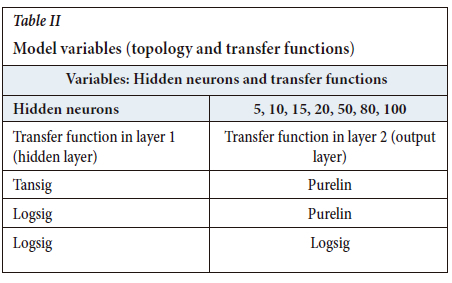
The topology and transfer function variables are summarized in Table II. Each ANN consists of an input, one hidden, and an output layer with a transfer function in the hidden and output layers. The number of neurons in the hidden layer was also varied.

 

 

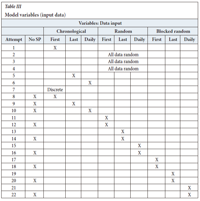
Lastly, the input data used to train the ANN was varied, as given in Table III and further explained in the subsection on data shuffling. The heading 'No SP' in this table describes neural networks where the set-point data (as shown in Table I) was not included as input to the ANN. Furthermore, 'Chronological' means that the input data to the ANN was in chronological order as the samples were taken and sensor data collected. The heading 'Random' refers to individual data shuffling (discussed in the subsection Data shuffling). Similarly, Blocked random refers to blocked data shuffling. Lastly, 'First', 'Last', and 'Daily' refer to the 70% training data being either the first 70% of the set, the last 70% of the set, or the last 70% of each sampling day, respectively.

For example, attempt 1 utilizes all of the 18 inputs as described in Table I. The input data consists of the first 70% of the chronological data-set. Furthermore, an ANN was trained using 5, 10, 15, 20, 50, 80, and 100 hidden neurons. For each of these configurations, the transfer function pair, as described in Table II, was also considered. Hence, one of the networks trained for attempt 1 will comprise 18 inputs, using 5 hidden neurons and a tansig transfer function in the hidden layer with a purelin transfer function in the output layer.

Data shuffling

In the first attempt, the data to the ANN is imported chronologically using the first 70% of the data (as shown in Table III). In this division, the minimum and maximum data-points are included in the training set, which is essential due to the poor extrapolation ability of neural networks (Hasson, Nastase, and Goldstein, 2020).

Furthermore, since the model does not receive dynamic data (such as a rate of change resulting from a dependency between data-points in a time sequence), data shuffling was investigated. It has been observed that data shuffling reduces overfitting, improves the testing accuracy and convergence rate, and results in better generalization of the neural network (Kaushik, Choudhury, Kumar, Dasgupta, Natarajan, Pickett, and Dutt, 2020, p. 2; Ke, Cheng, and Yang, 2018, p. 1; Nguyen, Trahay, Domke, Drozd, Vatai, Liao, and Gerofi, 2022, p. 1085). There are various methods to shuffle the data, including individual shuffling using shuffling algorithms, batch shuffling, etc. (Baheti, 2022). Shuffling can occur at different points during the training process. MatlabTM offers two main options: shuffling once before training starts (default) or after every epoch (MathWorks, 2022).

All data was shuffled during attempt 2, including the simulation data. However, the question arose whether shuffling impacted the results; hence attempts 3 and 4 were also performed. Another problem with these three attempts was that the actual plant data would not enter the ANN shuffled but rather chronologically as a data stream, and random shuffling is, therefore, not an accurate representation. Thus, attempts 2-4 are considered invalid and not repeated for different transfer functions.

The training data was grouped into three groups as follows (Table III):

1 Using the first 70% of the data

2 Using the last 70% of the data

3 Using the last 70% of each sample day's data (blocked shuffling).

These three groups of data were shuffled as follows:

1 Chronological data (no shuffling)

2 Random shuffling of only the training data (individual shuffling)

3 Grouping the data into sample blocks (blocked shuffling).

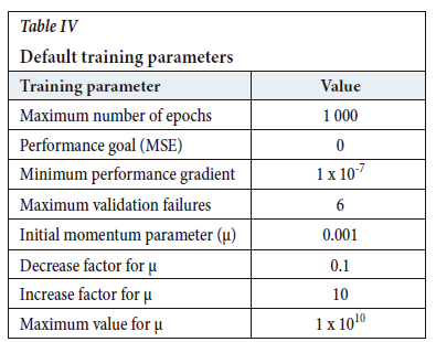
The default training parameters in Matlab^TM were used as given in Table IV. However, the weights and biases were initialized at 0.5 wso that all models could be compared from the same starting point.

 

 

Experimental methodology

Materials and sample preparation

Phosphogypsum samples were collected at the product bagging section of the plant after the calcining and milling processes. To determine the optimum sampling rate, the residence time of the plant is required. This residence time was determined at start-up: from when the feed conveyor belt started to when the first material reached the bagging section. Using the Nyquist sampling rate criterion, it was determined that the sampling rate should be half of the residence time (Landau, 1967).

The crucibles were engraved for identification purposes, cleaned, and dried in an oven. The cleaned crucibles were then left to cool in a desiccator, after which the mass of each was determined and recorded (M_c). A Mettler Toledo AB204-S/FACT analytical balance was used for this purpose. Lastly, 95% ± 0.15% ethanol was prepared from 99.99% ethanol.

Sampling

Hemihydrate samples were taken at the bagging section of the plant. The residence time of the plant was 20 minutes; so according to the Nyquist theorem, sampling should occur in 10 minute intervals (Landau, 1967). As the samples were taken and sealed in plastic containers, the time, date, and product bag number were recorded on the container. A portion of each sample was also taken and stored in a sealable bag for repeatability analysis. It is important to note that sampling could only occur once the plant was operating at a steady state, i.e. when normal operating conditions had been maintained for approximately 2 hours.

Sample analysis

Total bound moisture (TBM)

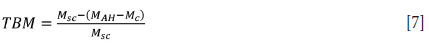
The TBM analyses were done by weighing and recording approximately 10 g of material in a crucible (Msc). The crucible name, sample, and mass of the sample were recorded. The samples were placed in a furnace (Carbolite Gero AAF 1100 and VMF 1000) at 450°C for 2 hours. The samples were then removed and allowed to cool in a desiccator. Finally, the mass of the dried sample (with the crucible) was recorded (MAH). The TBM was then calculated as follows:

Gypsum anhydrite

To determine the amount of gypsum anhydrite in the sample, 10 g of each sample was again weighed off, and the mass was recorded as M_sc. Then, approximately 10 ml of 95% ethanol was added to the sample, ensuring the sample was submerged in the liquid. Care was taken to ensure no spillages occurred as the liquid was swirled in the crucible. The hydrated sample was then placed in an oven at 45°C (Scientific Series 2000) for 24 hours. At this temperature, dehydration of the gypsum does not occur, and only surface moisture is removed (Li and Zhang, 2021). Furthermore, the anhydrite samples were dried for the same time as the hemihydrate samples for consistency. The crucible was then removed from the oven and allowed to cool in a desiccator. The mass of the sample and crucible was then recorded as M_sd.

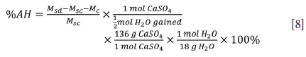
If the recorded mass of the sample (M_sc) was greater than the hydrated mass (M_sd - M_c), then weight loss occurred, which can be attributed to surface moisture in the sample; thus, no gypsum anhydrite was present. Alternatively, if a mass gain occurred (M_sc > M_sd - M_c), the water in the ethanol reacted with the soluble gypsum anhydrite and gypsum hemihydrate formed. The percentage of gypsum anhydrite (%AH) present in the sample can be calculated as follows:

The fraction of water gained by converting the anhydrite gypsum to hemihydrate gypsum is calculated as follows:

Gypsum hemihydrate

The same procedure as with the anhydrite analysis was followed to determine the amount of gypsum hemihydrate in the sample. However, the ethanol was replaced with ultrapure (Milli-Q) water. The fraction of water gained by converting the gypsum hemihydrate to gypsum dihydrate was determined using Equation [10] (note that any gypsum anhydrite will also react).

The percentage of gypsum hemihydrate (%HH) can then be calculated using Equation [11]:

Inert analysis

After the samples for the hemihydrate analysis had been weighed, the completely hydrated samples were further heated to 450°C for 4 hours. At this temperature, all the free moisture and crystal water is removed. The percentage of pure gypsum (%Purity) can then be calculated as the ratio between the actual mass of water gained vs. the theoretical maximum water gain.

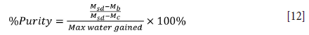
where

The percentage of impurities (%Inerts) in the sample can then be calculated as:

Gypsum dihydrate

The phase analysis was completed by a mass balance to determine the percentage of gypsum dihydrate (%DH) in the sample:

 

Results and discussion

TBM as a quality indicator

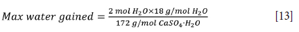
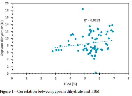
The correlation between gypsum dihydrate and TBM (Figure 1) was poor. The correlation between gypsum hemihydrate and TBM was significantly stronger (Figure 2). This is expected as a TBM analysis is commonly used to quantify a gypsum product's plaster (hemihydrate) content (ASTM Standard C 471M-01, 2017). The correlation between gypsum anhydrite and TBM is shown in Figure 3. An even stronger correlation can be observed. However, the slope of the regression plot is negative.

 

 

 

 

 

 

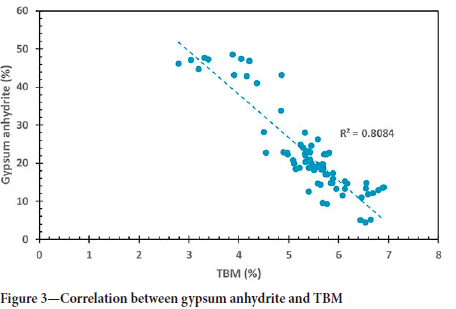
These correlations seem counterintuitive since one would expect the two phases with crystal water (gypsum dihydrate and gypsum hemihydrate) to correlate strongly with a bound moisture indicator. Instead, the strongest correlation with TBM is found with the gypsum anhydrite phase. These results are in accordance with an analysis done by the plant engineer. Unfortunately no explanation could be found for this observation, but additional studies are under way to understand this concept.

The industry target TBM of 5.8% was investigated. A gypsum hemihydrate content of between 60% and 80% was achieved at this TBM. Furthermore, the gypsum anhydrite content was 10-30%, and the gypsum dihydrate content was 4-14%. At this TBM, a large amount of gypsum hemihydrate is present, with a small amount of gypsum anhydrite and limited amounts of gypsum dihydrate. The low gypsum dihydrate content is desired since this indicates a large conversion from feed gypsum to useful gypsum hemihydrate. Furthermore, the quantity of gypsum hemihydrate should be maximized, with a small amount of gypsum anhydrite to improve setting times (Tzouvalas, Dermatas, and Tsimas, 2004). However, the gypsum anhydrite content should also be limited, otherwise flash settling might occur (Tydlitát, Medved', and Černý, 2012).

Artificial neural network

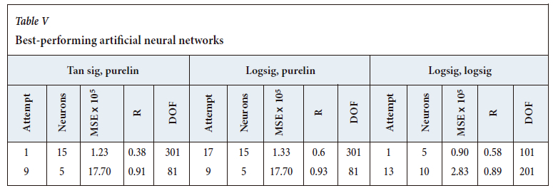
For each attempt and each run, the training, validation, testing, and simulation performance was documented using the mean squared error (MSE) and correlation coefficient (R). The performance is based on the lowest MSE and highest R-value for each attempt. The results indicated that the best run of the logsig-logsig configuration is still worse than the other two configurations, where the logsig-purelin configuration shows the best results.

The best-performing models for each of the transfer function pairs with respect to the two performance measures are shown in Table V. Of the six best networks, only two (attempt 9 of the logsig-purelin and tansig-purelin configurations) performed well when the set-point data was removed. Therefore, it can be concluded that the set-point data is valuable training information for the ANNs. A possible explanation for this is that the set-point offers a more constant value than the slightly deviated measurement. Additionally, a set-point change is immediate, whereas plant conditions have a slower response, and hence the model would 'see' and 'expect' a change. Furthermore, the chronological data also performed well, as seen in attempt 1 of the tansig-purelin and logsig-logsig configurations. Lastly, attempts 17 of the logsig-purelin and 13 of the logsig-logsig configurations also performed well. These two attempts consisted of data from the first two days of sampling with quite variable product quality and the 'stable' last day of sampling. Similarly, attempt 9 also consisted of data from all the days. This shows the importance of training the model using data that encompasses the characteristics of the entire data-set.

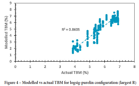
The hyperbolic tangent and log-sigmoid transfer functions are widely used for multilayer backpropagation networks (Dorofki et al., 2012; Hagan et al., 2014; Kriesel, 2007). The performance of each transfer function depends on the application thereof, as confirmed by Dorofki et al., (2012). This result was also seen in the application to the calciner, as the logsig-purelin topology seems to outperform the tansig-purelin topology. However, Kriesel (2007) states that it is essential that the output transfer function is linear, so as not to limit the output interval. This is also seen in the results obtained - the logsig-purelin topology outperforms the logsig-logsig topology. A parity plot of the logsig-purelin configuration is given in Figure 4.

 

 

Conclusions and recommendations

The industry operational target of 5.8% total bound moisture (TBM) is deemed sufficient. At this point, a gypsum dihydrate conversion of about 90% is achieved. Furthermore, gypsum hemihydrate makes up most of the product (about 70%), with a sufficiently small quantity of gypsum anhydrite (about 20%). Therefore, based on these results, the target TBM is sufficient to control the product quality. Furthermore, no offset between the calculated and experimental TBM was observed on the last day of sampling, which could be due to the stricter plant control. Lastly, no correlation was found between the purity of the gypsum product and the TBM. This indicates that impurities with crystal moisture were not present in significant amounts. Based on the simulation set of the first sampling campaign, the logsig-purelin configuration with the highest R-value provided the best performance. This model is sufficient to use as a control guideline since the coefficient of correlation is greater than 90%. The strength of the model is indicated by R² (86%)

Even though the TBM could be correlated to the gypsum phases, a more in-depth study is required. It is suggested that this study would look more at how the different phases impact product quality. For example, to what extent does gypsum anhydrite impact the setting time of the product? From this information, an optimum compositional range for each phase should be determined. This can then be used to calculate the desired TBM.

A more complex ANN topology and training structure should be investigated. Concerning the topology, different transfer function configurations should be investigated. The logsig-logsig configuration provided better results for the additional data, whereas the logsig-purelin configuration provided better results for the original data. It would be worthwhile to investigate the performance of different configurations, such as a tansig-logsig configuration. Furthermore, regarding the training structure, it is suggested that the performance of an optimized training algorithm, such as shuffling between each epoch, be investigated. In addition, the arbitrary decision of a 70:30 division between the training and simulation data could also be investigated. Lastly, a larger data-set would be beneficial to ensure sufficient data is available to obtain satisfactory training and simulation results.

 

Acknowledgements

We want to thank Mr R. van der Merwe and OMV Potchefstroom for answering all my questions regarding the plant and the gypsum process and allowing me to proceed with this work. Thank you also to Mrs R. Bekker for your unending help and patience in the laboratory.

 

Credit author statement

MJ: Conceptualisation, Methodology, Software, Investigation, Validation, Formal analysis, Writing, Visualization; FvdM: Supervision, Project administration, Funding acquisition, Reviewing; FHC: Supervision, Project administration, Funding acquisition, Reviewing; R-DT: Visualization, Reviewing.

 

References

Abraham, A. 2005. Artificial neural networks. Handbook of Measuring System Design. Sydenham, P.H. and Thorn, R. (eds). Wiley, London. pp. 901-908.         [ Links ]

Alwosheel, A., van Cranenburgh, S., and Chorus, C.G. 2018. Is your dataset big enough? Sample size requirements when using artificial neural networks for discrete choice analysis. Journal of Choice Modelling, vol. 28, no. 1. pp. 167-182. https://doi.org/10.1016/j.jocm.2018.07.002        [ Links ]

ASTM Standard C 471M - 01. 2017. Standard test methods for chemical analysis of gypsum and gypsum products. ASTM International, West Conshohocken, PA.         [ Links ]

Azadi, S. and Karimi-Jashni, A. 2016. Verifying the performance of artificial neural network and multiple linear regression in predicting the mean seasonal municipal solid waste generation rate: A case study of Fars province, Iran. Waste Management, vol. 48. pp. 14-23.         [ Links ]

Baheti, P. 2022, Train test validation split: how to & best practices [Blog post]. https://www.v7labs.com/blog/train-validation-test-set [accessed 5 October 2022].         [ Links ]

Brezak, D., Bacek, T., Majetic, D., Kasac, J., and Novakovic, B. 2012. A comparison of feed-forward and recurrent neural networks in time series forecasting. Proceedings of the 2012 IEEE Conference on Computational Intelligence for Financial Engineering & Economics (CIFEr), Croatia. https://ieeexplore.ieee.org/stamp/stamp.jsp?tp=&arnumber=6327793        [ Links ]

Cave, S. 2000. Gypsum calcination in a fluidised bed reactor. PhD thesis, Loughborough University, UK.         [ Links ]

Christensen, A.n., Olesen, M., Cerenius, Y., and Jensen, T.R. 2008. Formation and transformation of five different phases in the CaSO₄-H₂O system: crystal structure of the subhydrate ß-CaSO₄-0.5 H₂O and soluble anhydrite CaSO4. Chemistry of Materials, vol. 20, no. 6. pp. 2124-2132. https://doi.org/10.1021/cm7027542        [ Links ]

Dantas, H., Mendes, R., Pinho, R., Soledade, L., Paskocimas, C., Lira, B., Schwartz, M., Souza, A., and Santos, I. 2007. Characterisation of gypsum using TMDSC. Journal of Thermal Analysis and Calorimetry, vol. 87, no. 3. pp. 691-695. https://doi.org/10.1007/s10973-006-7733-9        [ Links ]

Dorofki, M., Elshafie, A.H., Jaafar, O., Karim, O.A., and Mastura, S. 2012. Comparison of artificial neural network transfer functions abilities to simulate extreme runoff data. Proceedings of the 2012 International Conference on Environment, Energy and Biotechnology. International Association of Computer Science and Information Technology Press, Singapore. pp. 39-44.         [ Links ]

Gürsel, D., Möllemann, G., Clausen, E., Nienhaus, K., and Wotruba, H. 2021. Online measurements of material flow compositions using acoustic emission: Case of gypsum and anhydrite. Minerals Engineering, vol. 172, no. 1. pp. 1-10. https://doi.org/10.1016/j.mineng.2021.107131        [ Links ]

Hagan, M.T., Demuth, H.B., Beale, M.H., and Jesus, O.D. 2014. Neural network design. https://hagan.okstate.edu/NNDesign.pdf [accessed 12 October 2022]        [ Links ]

Hasson, U., Nastase, S.A., and Goldstein, A. 2020. Direct fit to nature: an evolutionary perspective on biological and artificial neural networks. Neuron, vol 105, no.3. pp. 416-434.         [ Links ]

Heaton, J. 2008. Introduction to Neural Networks with Java. 2nd edn. Heaton Research, Inc., Chesterfiel, MO.         [ Links ]

Jordan, L.A. and van Vuuren, D. 2022. Heat-constrained modelling of calcium sulphate reduction. Journal of the Southern African Institute of Mining and Metallurgy, vol. 122, no. 10. pp. 607-616. http://dx.doi.org/10.17159/2411-9717/1530/2022        [ Links ]

Kaushik, S., Choudhury, A., Kumar, P.K., Dasgupta, N., Natarajan, S., Pickett, L.A., and Dutt, V. 2020. AI in healthcare: time-series forecasting using statistical, neural, and ensemble architectures. Frontiers in big data. pp. 1-17. doi.org/10.3389/fdata.2020.00004        [ Links ]

Kavzoglu, T. and Mather, P.M. 2003. The use of backpropagating artificial neural networks in land cover classification. International Journal of Remote Sensing, vol. 24, no. 23. pp. 4907-4938. https://doi.org/10.1080/0143116031000114851        [ Links ]

Koper, A., Pralat, K., Ciemnicka, J., and Buczkowska, K. 2020. Influence of the calcination temperature of synthetic gypsum on the particle size distribution and setting time of modified building materials. Energies, vol. 13, no. 21. 5759. https://doi.org/10.3390/en13215759        [ Links ]

Krenker, A., Bester, J., and Kos, A. 2011. Introduction to the artificial neural networks. Artificial Neural Networks: Methodological Advances and Biomedical Applications. Suzuki, K. (ed.). InTech, Croatia. pp. 1-18.         [ Links ]

Kriesel, D. 2007. A brief introduction to neural networks. http://www.dkriesel.com/en/science/neural_networks [accessed 12 October 2022].         [ Links ]

Landau, H. 1967. Sampling, data transmission, and the Nyquist rate. Proceedings of the IEEE, vol. 55, no. 10. pp. 1701-1706. https://doi.org/10.1109/PROC.1967.5962        [ Links ]

Li, X. and Zhang, Q. 2021. Dehydration behaviour and impurity change of phosphogypsum during calcination. Construction and Building Materials, vol. 311, no. 13. pp. 1-10. https://doi.org/10.1016/j.conbuildmat.2021.125328        [ Links ]

Lourakis, M.I. 2005. A brief description of the Levenberg-Marquardt algorithm implemented by levmar. Foundation of Research and Technology, vol. 4, no. 1. pp. 1-6.         [ Links ]

May, R., Dandy, G., and Maier, H. 2011. Review of input variable selection methods for artificial neural networks. Artificial Neural Networks -Methodological Advances and Biomedical Applications. InTech, Rijeka, Croatia. pp. 19-44.         [ Links ]

Mechchem Africa. 2019. Gypsum reprocessing for a cleaner environment. https://www.crown.co.za/latest-news/mechchem-africa-latest-news/10236-gypsum-reprocessing-for-a-cleaner-environment [accessed 28 July 2022].         [ Links ]

Nguyen, T.T., Trahay, F., Domke, J., Drozd, A., Vatai, E., Liao, J., and Gerofi, B. 2022. Why globally re-shuffle? Revisiting data shuffling in large scale deep learning. 2022 IEEE International Parallel and Distributed Processing Symposium (IPDPS). IEEE. pp. 1085-1096.         [ Links ]

Rajković, M., Tošković, D., Stanojević, D.D., and Lačnjevac, Č. 2009. A new procedure for obtaining calcium sulphate α-hemihydrate on the basis of waste phosphogypsum. Journal of Engineering & Processing Management, vol. 1, no. 1. pp. 99-113.         [ Links ]

Ranganathan, A. 2004. The levenberg-marquardt algorithm. https://sites.cs.ucsb.edu/~yfwang/courses/cs290i_mvg/pdf/LMA.pdf [accessed 28 Jul 2022].         [ Links ]

Rudd-Orthner, R.N. and Mihaylova, L. 2021. Deep ConvNet: Non-random weight initialization for repeatable determinism, examined with FSGM. Sensors, vol. 21, no. 14. pp. 4772. https://doi.org/10.3390/s21144772        [ Links ]

Saadaoui, E., Ghazel, N., Ben Romdhane, C., and Massoudi, N. 2017. Phosphogypsum: potential uses and problems - a review. International Journal of Environmental Studies, vol. 74, no. 4. pp. 558-567. https://doi.org/10.1080/00207233.2017.1330582        [ Links ]

Seufert, S., Hesse, F., Goetz-Neunhoeffer, G., and Neubauer, J. 2009. Quantitative determination of anhydrite III from dehydrated gypsum by XRD. Cement and Concrete Research, vol 39, no. 1. pp. 936-941. https://doi:10.1016/j.cemconres.2009.06.018        [ Links ]

Sheela, K.G. and Deepa, S.N. 2013. Review on methods to fix number of hidden neurons in neural networks. Mathematical Problems in Engineering. Article 425740. https://www.hindawi.com/journals/mpe/2013/425740/        [ Links ]

Singh, N. and Middendorf, B. 2007. Calcium sulphate hemihydrate hydration leading to gypsum crystallisation. Progress in Crystal growth and Characterisation of Materials, vol. 53, no. 1. pp. 57-77. https://doi.org/10.1016/j.pcrysgrow.2007.01.002        [ Links ]

Tydlitát, V., Medved, I., and Černý, R. 2012. Determination of a partial phase composition in calcined gypsum by calorimetric analysis of hydration kinetics. Journal of Thermal Analysis and Calorimetry, vol. 109, no. 1. pp. 57-62. https://doi.org/10.1007/s10973-011-1334-y        [ Links ]

Tzouvalas, G., Dermatas, N., and Tsimas, S. 2004. Alternative calcium sulfate-bearing materials as cement retarders: Part I. Anhydrite. Cement and Concrete Research, vol. 34, no. 11. pp. 2113-2118. https://doi.org/10.1016/j.cemconres.2004.03.020        [ Links ]

Wilamowski, B.M. 2011. Neural networks learning. Industrial Electronics Handbook. Wilamowksi, B.M. and Irwin, J.D. (eds). Taylor & Francis, Florida. pp 11-1 - 11-18.         [ Links ]

Yu, H. and Wilamowski, B.M. 2011. Levenberg-Marquardt training. Industrial Electronics Handbook: Intelligent Systems. Wilamowksi, B.M. and Irwin, J.D. (eds). 2nd edn. Taylor & Francis, Florida. pp 12-15.         [ Links ]

Zhang, G., Patuwo, B.E., and Hu, M.Y. 1998. Forecasting with artificial neural networks: The state of the art. International Journal of Forecasting, vol. 14, no. 1. pp. 35-62. https://doi.org/10.1016/S0169-2070(97)00044-7        [ Links ]

 

 

Correspondence:
M. Jacobs
Email: marlisejacobs71@gmail.com

Received: 29 Nov. 2022
Revised: 7 Sept. 2023
Accepted: 21 Sept. 2023
Published: October 2023

 

 

* Paper written on project work carried out in partial fulfilment of BEng (Chemical Engineering with Specialisation in Minerals processing) degree