PROFESSIONAL TECHNICAL AND SCIENTIFIC PAPERS

 

Predicting open stope performance at an octree resolution using multivariate models

 

 

B. McFadyen^I; M. Grenon^I; K. Woodward^II; Y. Potvin^II

^IUniversité Laval, Département de génie des mines, de la metallurgie et des matériaux, Canada. ORCID: M. Grenon: http://orcid.org/0000-0003-3919-9275
^IIAustralian Centre for Geomechanics, The University of Western Australia, Australia

Correspondence

 

 

---

SYNOPSIS

Open stoping has become a popular mining method in hard rock mines, not only due to the safety of the method as a non-entry approach, but also because of the high extraction rate and low costs. At mine sites, stope performance is evaluated by calculating stope overbreak using the stability chart. However, limitations of the stability chart regarding the precision of the predictions, non-consideration of factors such as the influence of blasting, and the exclusion of underbreak have led to non-optimal designs. The capabilities of today's computers have increased the amount of data being collected and the power of models being built. This article presents a step towards a new stope design approach where stope overbreak and underbreak are measured and georeferenced using octrees at an approximately cubic metre resolution and predicted using multivariate statistical models (partial least square, linear discriminant analysis, and random forest). Results show that overbreak and underbreak location along the design surface and their magnitude are predicted with good precision using a random forest model. These predictions are used to build the expected geometry of the open stope. The resolution of the data and the use of multivariate analysis has enabled the prediction of variation in stope performance along the design surface, going well beyond the simple qualitative per stope face prediction provided by a traditional stability chart approach.

Keywords: stope design, stope reconciliation, overbreak, underbreak, multivariate, prediction, random forest.

---

 

 

Introduction

When designing and mining an open stope, the goal is to create a final void geometry which is stable and closely matches the designed geometry. However, what commonly occurs when extracting open stopes is the unintentional mining of volumes of overbreak (OB; rock or backfill material mined outside of the design volume) and underbreak (UB; rock in the design volume left behind). This can have a strong operational and economic impact on the mine as it can cause stability issues which extend to the adjacent mining excavations, dilution of ore with waste material, the loss of ore reserves that are no longer recoverable, or problems at the mill which is optimized for expected grades and rock chemistry. Therefore, identifying the root cause factors of stope OB and UB enables the mine's engineers to understand stope performance. This knowledge is then used when designing open stopes to minimize stope OB and UB and to maximize the value realized from mining.

The stability chart is a popular predictive tool used in current stoping practices (Mathews et al., 1981; Potvin, 1988; Nickson, 1992). This chart is an empirical and bivariate tool that qualitatively predicts the stability of a stope face and assesses a stability number, which is calculated from the geomechanical properties of the rock mass and the hydraulic radius, which is derived from the planned geometry. Based on the results, a decision is made regarding stope dimensions or the need for ground support. Once mining has started, the use of the stability chart as an optimizing tool is limited as it does not quantify operational parameters that can be modified for optimizing stope performance, e.g. blasting parameters. The stability chart is not capable of assessing UB, which is largely controlled by operational parameters not considered by the method. Therefore, the use of the stability chart is best suited at the feasibility stage (or the life-of-mine stope planning step) when the approximate dimensions of the stopes and sequence need to be decided.

Site-specific tools can also be developed using their own reconciliation data. However, workshops conducted in Australia and Canada in 2019 highlighted that root cause analysis is done for OB at all participating mine sites, but only some mines do it for UB. Furthermore, they still use the stability chart developed over 40 years ago to assess stope stability and do not use any tools to predict UB (Potvin et al., 2020). Important parameters that have a major impact on the stope performance, such as faults, undercut, stand-up time, and blasting, are not considered in the standard stability chart (Clark and Pakalnis, 1997; Wang, 2004; Potvin et al., 2016; Guido, Grenon, and Germain, 2017; McFadyen, 2020). Despite the evolution of technology increasing the amount and type of data collected at mine sites and the computational methods for quantifying these parameters, these parameters are not currently used for prediction of stope performance.

The common mining practices described above highlight the need for developing a new stope design approach that incorporates the different parameters critical to stope Ob and UB in order for mines to understand, predict, and optimize stope performance at the design stage. A novel approach to predict and optimize the outcome of a planned stope can be developed, thanks to a combination of increased computational capabilities, powerful multivariate statistical analysis (Guido and Grenon, 2018; McFadyen, 2020), and reconciliation tools at a significantly finer resolution (Woodward et al., 2019).

Building towards a new stope design methodology, this paper will show how multivariate statistics and data measured at an approximately cubic metre resolution (referred to here as octrees) is used to predict stope performance, giving information and knowledge at the design stage for the optimization of stope performance and mine planning. This approach presents many novelties due to the resolution of the analysis (per octree) and the wide range of parameters considered which are known to impact stope performance. Georeferenced points along the design surface are efficiently obtained with the octree data structure, providing much better predictions and spatial representation of stope OB and UB compared to a per-face prediction. This research represents a significant leap for the capability of mine sites to optimize stope performance at the design stage. The following work details the statistical analysis approach and presents the results of a case study.

 

Literature review

The stope design process can be divided into four main steps

(Potvin et al., 2020):

> Life-of-mine stope planning

> Stope design

> Operation and execution

> Reconciliation.

Predicting stope performance is an empirical process that utilizes information gathered from the final reconciliation step to develop a tool that can be integrated into the first two steps of the design process. Stope reconciliation compares the design and mined geometry to quantify the OB and UB (Figure 1).

 

 

This step is typically done at two levels of resolution, on a per-stope and per-face basis. The total volume and percentage are quantified and, at a per-face resolution, the linear equivalent overbreak slough first introduced by Clark, 1998 (ELOS; Figure 2) and the linear equivalent loss ore (ELLO) are also quantified.

 

 

The mined surface is generated by a cavity monitoring system scan (CMS; Miller, Potvin, and Jacob, 1992). A CMS uses a laser rangefinder mounted on a head that tilts and rotates 360° to survey a cavity from one of the entry points. The scan generates a point cloud which can then be meshed for analysis. The resolution will depend on the density of points set by the surveyors. Multiple CMS scans can be done at different times to follow the evolution of the void. However, the CMS used for the reconciliation is the final scan done once mucking is finished. The accuracy is typically 2 cm, but the scan can be affected by external factors such as fog, dust, ground support mesh, or irregular surfaces. These will cause shadowed areas for part of the stope, preventing adequate interpretation of the actual geometry. It is possible to get around these limitations by doing multiple scans from different entry points.

The predictive tools can be based on the mine's own data as mining progresses or on a stope database built from other mines that employ similar methods and have analogous conditions. The latter approach is comparable to the stability chart (Figure 3), which is the most widely used predictive tool at the life-of-mine stope planning step. The stability chart qualitatively estimates OB on a per-face basis. This tool is well adapted for this step as no reconciliation data is available from the mine and only geomechanical and geometrical data are quantified. The stability chart is also commonly used at the stope design stage, although it does not offer possibilities for optimization.

 

 

As stope extraction progresses, data from the reconciliation of the mined stopes becomes increasingly available and can be used to develop a site-specific predictive tool. These tools use a statistical approach for a given resolution of reconciled data. Existing predictive tools generate predictions on a per-face basis, as this is the finest resolution being processed for most mines (Potvin et al., 2020). Mines generally predict an OB volume as the ELOS using parameters averaged over the whole face. They also tend to focus on specific faces such as the hangingwall (Potvin et al., 2020). UB tends to not be considered during these assessments. A new and finer detailed reconciliation process where data is reconciled on a per-octree basis allows for a more refined and complete prediction (Woodward et al., 2019).

Octrees represent georeferenced blocks which cover the design and mined three-dimensional (3D) space. A finer resolution of blocks is obtained along the design and mined surfaces by recursively subdividing the 3D space until the desired size or resolution of the octrees (usually < 1 m) is obtained (Figure 4). The stope performance is quantified for each octree block on the design surface by calculating a projected distance, which is defined as the distance in the direction normal to the design between the design and mined surfaces. Positive values represent OB while negative values represent UB.

 

 

Different statistical methods exist for building a predictive model. The ability of a model to generate accurate predictions will depend on the type of data and its distribution, along with the relationship between the parameters. The statistical model can be obtained by using a supervised method, which means, in this specific case, the stope performance data is used for building the model. The method used to build the model can be linear, discriminant, tree-based, additive, or a neural network (Hastie et al., 2017). The model can also be obtained using an unsupervised method, meaning, in this specific case, the stope performance is not considered when building the model but can be used later to analyse the applicability of the model to distinguish stope performance. These methods are usually based on cluster analysis or principal component analysis (Hastie et al., 2017).

Current statistical approaches for predicting stope performance vary from a bivariate to a multivariate decision-making process. In all cases, a supervised method is used to calculate the predictions, but some do utilize concepts of unsupervised methods to create the charts used for predictions. The stability chart is a bivariate approach, where the decision is made from two parameters (stability number and hydraulic radius). The different zones (stable, unstable, caving) can be separated using a discriminant method (Nickson, 1992). Mines can also create their own bivariate chart if the critical parameters are known and quantified. However, these tend to be limited in terms of predictive capabilities since there is most likely more than one critical parameter affecting stope performance. A multivariate approach is therefore the most suitable method for generating accurate predictions. Multiple linear regression (MLR; Wang, 2004; Hughes, 2011; Guido and Grenon, 2018) and principal component logistic regression (PCR; Guido and Grenon, 2018) were shown to improve the OB predictions accuracy over the stability chart on a per face basis. McFadyen (2020) has shown that a partial least square model (PLS) can be used to generate accurate predictions of OB in the hangingwall. Random forest (Breiman, 2001) was used by Qi et al. (2018) and an artificial neural network (McCulloch and Pitts, 1943) was used by Adoko et al. (2022) to classify a face OB performance using geometrical and geomechanical parameters.

 

Methodology

This article proposes a new empirical stope design approach to help engineers with optimizing stope performance. This approach uses data at an octree resolution to understand (through multivariate statistical analysis) and predict (through a multivariate statistical model) stope performance at the mine site. The methodology for understanding and identifying the critical parameters using multivariate analysis is detailed in McFadyen et al. (2023). The critical parameters are used for predicting stope performance on a point basis, giving detailed and spatial information of the OB and UB. Furthermore, this allows for the generation of a predicted shape of the final void (referred to as 'predicted CMS' in this article). The acquired knowledge and predicted CMS can then be used during stope design for optimization and planning. This article details the prediction process from building to validating the models.

Octree data

The new stope design approach is based on data being quantified and reconciled at an octree resolution. Using this resolution means we are quantifying and predicting the spatial variation of the stope performance along the designed stope shape. Figure 5 gives an example of the spatial variation of stope performance captured using octrees. For this example, predicting on a per-face basis would give the thickness of OB and UB (ELOS and ELLO), but would not allow identification of where the OB and UB would occur in the face, or the magnitude of OB or UB in specific locations. Using octrees, the stope performance is measured at thousands of georeferenced points, spatially capturing where OB and UB occur, as well as the spatial distribution of the parameters being analysed. We can therefore predict the magnitude of OB or UB in specific locations across the designed stope surface.

 

 

Another advantage of using data quantified at an octree resolution is that geometrical, geological, geomechanical, and operational parameters can be quantified, offering a wider range of parameters that can be considered than on a per-face basis. It also allows for optimization as operational parameters such as blasting can be integrated into the model.

Multivariate predictive model

Multivariate statistical models are used to generate the predictions. These models use multiple input parameters and previously mined stope data to predict the performance of the future stopes. While many different models exist, three models were tested and are discussed in this paper: PLS (Wold, 1966), linear discriminant analysis (LDA; Fisher, 1936), and random forest (Breiman, 2001). PLS is a linear approach that quantifies the covariance between the input parameters and stope OB and UB in order to make predictions. LDA is a discriminant approach that aims to correctly classify the octrees as OB or UB (for this paper) by finding the axis that best separates the two. Random forest is a tree-based method where multiple trees are generated to obtain a predictive value.

These models were selected due to previous use and performance on a per-face basis (PLS: McFadyen, 2020, and LDA: Nickson, 1992) as well as the random forest model's ability to capture a complex data structure. The three models were developed through the free software environment R (R Core Team, 2021). PLS used the PLS package (Liland et al., 2020), LDA used the MASS package (Venables and Ripley, 2002), and random forest used the Ranger package (Wright and Ziegler, 2017).

Statistical evaluation of model performance

The data is separated chronologically into three groups to test the quality of the models during their construction. The first group represents the first 50% of the data, the second represents the following 25%, and the final group represents the final 25% of the data. This approach enables the user to train a model with the first group of data and then test the predictive performance on the second group, optimize the model variables and finally predict the third group of data. This allows verification of whether the model generates accurate predictions and determines which model is best suited for the data-set, all while minimizing overfitting by the model.

When evaluating the model's statistical predictive performance, there are two aspects to consider. First, is whether an octree is correctly predicted as OB or UB, and secondly, is the predicted distance close to the actual projected distance. Based on the model's performance, the parameters can be analysed to understand their relationship with OB and UB.

For the first case, the capacity of the model to correctly predict if OB or UB is generated at the octree's location is measured by using the confusion matrix presented in Table I. This table separates the data into four categories, allowing the user to evaluate the error rate for OB and UB.

 

 

Different performance metrics will be calculated, such as the accuracy (percentage of octrees correctly predicted), the precision (percentage of overbroken octrees predicted as OB), the sensitivity (percentage of OB predictions that are correct), and the specificity (percentage of UB predictions that are correct). Each of these metrics evaluates a specific quality of the model. There is also the Matthews correlation coefficient (MCC; Matthews, 1975), which is a more complex metric but gives a global measure of the quality of the classifications, with 1 being perfect predictions, 0 being random, and -1 being all wrong predictions. Table II gives the equations for these metrics.

 

 

For the second case, the error of the prediction is measured by calculating the difference between the predicted value and the actual value of the projected distance for the octree. The overall root mean square error (RMSE) will be calculated from the predicted and observed distances as well as the distribution of the absolute value of the errors. This allows calculation of the percentage of octrees for which the predictions are within a certain distance. In the case of stope performance, six brackets have been established, as shown in Table III. These brackets have been determined using engineering judgement to characterize the spread in the accuracy.

 

 

It is also possible to evaluate the accuracy of the prediction by plotting the predictions versus the actual values for each octree. A perfect model would have the predictions follow a linear trend with all the points falling on a 45° line, meaning the predicted CMS would look exactly like the actual CMS. This rarely occurs due to the inherent uncertainty of measuring causative factors arising from the complexity of the underground geological and mining environment where the variation in the geomechanical properties of the rock mass, as well as the variation between the mined and planned data, cannot be fully captured. Furthermore, blasting is not a precise cutting tool compared to a tunnel-boring machine, implying some uncertainty around the final excavation geometry. A linear regression fit will be passed through the data to visualize the general trend of the predictions. The coefficient of determination (R²) will also be calculated to analyse the statistical quality of the regression. While the slope for the best linear fit in the data may not match the slope of the linear fit for a perfect model, it does not mean the predictions cannot be used at the design stage. The predictions can still indicate where OB and UB will likely occur and the expected magnitude. The reduced statistical significance arises from the model not precisely estimating the magnitude of the expected OB and UB. A visual analysis should be done in the end by comparing the predictions with the actual stope OB and UB to evaluate the performance of the model as the statistical evaluation does not describe spatial performance.

 

Case study

The Dugald River Pb-Ag mine is located in Queensland, Australia (Figure 6). Longitudinal and transversal stopes are used to extract the ore. Stope dimensions will vary depending on the area of the mine, but stopes are around 25 m high, between levels, and 15 m to 30 m long (Hassell et al., 2015). Stope widths vary between 2 m and 35 m depending on the orebody thickness. The orebody reaches a depth of approximately 1 km.

 

 

Data overview

This article focuses on 49 transversal stopes mined between 2017 and 2020 (Figure 7a). Each stope is reconciled on a per-stope, per-face, and per-octree basis. Drifts are cut out of the design and CMS geometry by site personnel during the building and processing of the geometries. For this reason, stope faces identified as drift surfaces (floors and crown mostly) are excluded from the analysis. Additionally, stope faces that are mined against backfill are excluded from analysis due to their vastly different strength and stress conditions. The 49 transversal stopes were separated into three groups chronologically. The first group contained 24 stopes, the second 13 stopes, and the last 12 stopes. The models were built using data from the first group, which consisted of 200 000 points, representing half the database. Since the final testing of the model was done with the final group, the results for group 3 will be presented (Figure 7b).

 

 

The parameters included in the analysis are presented in Table IV. These parameters correspond to the critical parameters idwentified in McFadyen et al., 2023 while assessing stope performance. Absent data occurs for the structural parameters since not all stopes have a fault in their vicinity. A maximum of 30 m between the fault and octrees is used in order to compute the distance and angle to fault. This distance was set based on the work by Woodward et al., (2019). For octrees with absent fault data a value must be given to include these octrees in the model since the model does not tolerate absent data. An arbitrary choice of a distance of 40 m is set and an angle of 100° in order to separate them from the octrees with fault data and keep them in the model.

 

Results

The overall statistical performance of the three predictive models is presented in Table V. Comparing the models, the random forest model performs better than the LDA and PLS based on the capacity to correctly predict octrees as OB and UB (67%) and the prediction error. It has a higher MCC (0.3) and a higher portion of octrees with a prediction error smaller than 0.5 m (39%) and 1 m (65%). Based on these statistical metrics, the random forest model performs well at predicting where OB and UB will occur as well as its magnitude, and would bring beneficial insight to the engineers.

 

 

After evaluating the statistical performance of the model, the predictions and the observations were visually compared in 3D space on the design surfaces. This innovative method predicts the detailed geometry of the expected void and allows for comparison of the spatial variation of the predictions to the actual CMS geometry. This is important as it will enable local verification of whether the predicted OB or UB matches the stope OB and UB. It also allows verification if the predictions would help the engineers in their decision-making since the prediction location is not considered in the statistical verification of the model's performance. Overall, with the PLS model, around 50% of the faces predicted would lead the engineer to the right interpretation of the location of OB and UB in the face based on the visual comparison of the predictions with the observed projected distance (location and magnitude of OB and UB). Good and bad prediction examples will be provided later in this paper. Similar to the PLS method, around 50% of the faces predicted with the LDA model would lead the engineer to the right interpretation of the location of OB and UB in the face. This assessment is based on a side-by-side visual comparison of the predictions with the observed projected distance for each face. These results indicate little benefit of the PLS and LDA models in stope design as the results are as likely to be wrong as right. For the random forest, around 75% of the faces predicted would lead the engineer to the right interpretation of the location of OB and UB in the face based on the visual comparison. The success rate of the random forest model indicates that stope OB and UB are predicted at an octree resolution using a more complex statistical model with good confidence. Given the superiority of the random forest model at predicting stope performance, the following section will further explore the results of the model in order to give visual examples and discuss the accuracy, probabilities, and limitations of the approach.

Random forest

Predictions from the random forest model represent the average prediction of all trees in the model (Figure 8). The model performance is optimized for a given data-set by varying the number of trees generated, the number of parameters randomly picked at each node (from which, based on a specified criterion, the parameter that maximizes the separation of the stope performance is then selected for that node), and the weight of octrees with a large predicted distance (over 2 m OB or UB) when randomly picking the octrees used for each tree due to the lower frequency of these distances. Preliminary testing of these three variables was done using the second group of stopes to obtain the most accurate predictions possible with this method. Based on the preliminary testing, the model is built using 500 trees, randomly picking two parameters at each node and assigning a 3:1 weight ratio to the larger projected distances to ensure an accurate representation. This model was used for the prediction of the stopes in group 3 and to evaluate its performance.

 

 

Statistical performance overview

The predictions generated for group 3 are plotted against the observations in Figure 9. The points have been coloured according to their confusion matrix classification. Linear regressions have been overlaid, with the blue line representing the ideal linear fit for predictions and the red line representing the best linear fit that is obtained from the predictions. The linear regressions help show that the data does have a linear trend, but the slope is smaller than what is desired.

The statistical metrics presented in Table V indicates the octrees were correctly predicted as OB or UB 67% of the time. This means 67% of the design surface would be accurately depicted as OB or UB. The MCC value is 0.3, meaning the classification is not perfect (MCC = 1), but is not random either (MCC = 0), indicating the selected parameters are critical for determining where OB and UB will occur and the model allows the user to make the distinction between the two. The model performs better at predicting if an octree is underbroken (70%) compared to overbroken (57%). The RMSE is 1.26, meaning the average error is around 1.26 m. The distribution of the prediction error indicates that just under 40% of the octrees are predicted within 0,5 m of the actual projected distance, 65% under 1 m, and 88% under 2 m. Given that the median is under 1 m error, the higher average error is due to localized areas of the stope where OB or UB is underpredicted.

Also, given the prediction error distribution, when looking at the predicted stope surface it can be assumed that most of the surface is within 1 m of its actual position and the majority within 2 m. Knowing that the stope performance has a range of 10 m (projected distance between -4 m and 6 m), the model allows the expected value range to be decreased to 1 to 2 m much of the time and up to 4 m for the majority of instances. The practical outcomes of these projected distances for a 25 χ 20 χ 20 m stope with a 0.5 m error across the whole stope would represent 1250 m³ error on the final volume (or 12.5%), while a 2 m error would represent 5000 m3 error on the final volume (or 50%). This volume is, however, separated between OB and UB. Overall, the random forest model with the selected critical parameters at an octree resolution has enabled us to determine where OB and UB will occur for the majority of the surface, as well as the projected distance within 1 m in many cases, and 2 m for the majority. These are considered significant contributions to prediction of stope performance, as the following visual example and probabilities will show.

Visual example

To better visualize the quality and accuracy of the predictions, a stope example (stope A) is presented for which the predictions match the statistical results presented in Table V and discussed in the previous section. Figure 10 presents two views of stope A, showing the actual values, the predictions, and the prediction error side-by-side. The visual example shows that the statistical accuracy of the model allows visual depiction of where OB and UB will occur and in the most part, the magnitude. The following conclusions are drawn from this figure.

> The model predicts that the bottom of the hangingwall will be underbroken and the top part overbroken. The sidewall will be overbroken for the most part. The bottom of the footwall will be overbroken and the top part underbroken. UB will be observed in most of the corners.

> When compared with the actual CMS, we observe a similar trend overall, predicting OB where there will be OB and UB where there will be UB.

> The main difference between the predictions and the actual values is in the prediction of large magnitudes of OB and UB (over 2 m or under 1 m). As we can see from the prediction error (areas with errors over 2 m), the predictions underpredict the OB or UB.

> These discrepencies occur, for the most part, towards the side of the stope that is against backfill, which is not taken into account in the model. The probabilities discussed in the next sections will provide further information.

Model accuracy

The overall accuracy of the model indicated in Table V and the visual analysis indicate reliable results can be obtained for predicting stope performance through a random forest model using the critical parameters identified at the mine site. Further analysis indicates that the accuracy of the model will vary depending on the observed projected distance. Figure 11 shows that the majority of octrees with a projected distance between -2 m and 2 m have smaller errors than larger distances. This is due in part to the fact that there are fewer octrees with a projected distance over 2 m and under -2 m. Since the predictions from random forest are the result of averaging, they are less sensitive to extreme values and can underpredict the larger projected distances. However, for each prediction, the standard error is calculated as the standard deviation of the predictions based on the prediction of each tree. A probabilistic approach is therefore used to assess larger OB and UB.

 

 

Probabilistic approach

From the standard error and predicted value, the probability density function (PDF) is obtained as well as the probability density curve. A normal distribution is assumed in this case. Using the PDF, we calculate the probability of observing a given value or the probability that an octree's projected distance will be larger or smaller than a specified distance. We also calculate a prediction interval within which the projected distance of the predicted octree is most likely to be for a given level of confidence. This means that for a level of 95% (calculated using the standard score), there is a 95% probability that the actual projected distance will be within the interval based on the model and selected observations.

Figure 12 shows the observed projected distance and the 60% prediction interval. The upper bound represents a probability that 80% of the projected distance will be smaller than this value and the lower bound represents a probability that 80% of the projected distance will be larger. These limits highlight the possibilities of large OB and UB. The projected distance of 63% of the octrees falls within the maximum and minimum projected distance values of the 60% prediction interval. Large OB can be expected in the hangingwall and UB in the bottom of the hangingwall and top of the footwall. Octrees that fall within the interval are also highlighted. In addition to the observations made in Figure 8, the probabilistic approach allows the user to determine that the hangingwall will likely see OB over 2 m, the top of the footwall ,UB over 2 m and the top of the bottom drive in the sidewall will see OB over 1.5 m. Since the location is not considered in the model, adjacent octrees can show a different prediction interval. In such cases, engineering judgement should be used for interpreting these predicted distances.

Given the standard error of the predicted octree, the probability of observing the predicted value will vary (the probability decreases as the standard error increases) and reflects the level of confidence we can attribute to the prediction. Figure 13 shows the binned cumulative probability of the predicted projected distances versus the prediction error. The prediction error increases when the probability of observing the predicted distance decreases, indicating the model's confidence in the prediction (higher probability), reflects the accuracy that can be expected based on the probability of the prediction. Small probabilities (larger standard error) for octrees are observed when some of the trees in the model will predict a wide range of projected distance. This would mean large and small OB or UB has been observed previously for octrees with similar parametric values, and therefore the probability of large OB or UB is higher for these octrees and hence the standard error is larger. The probability groups merge into one line for prediction errors over 4 m. These errors are associated with octrees with large OB and UB distances and can be due in part to the model averaging; and also to the fact that the selected parameters do not fully capture the cause for these large OB and UB distances and that some critical parameters do not match the reality or are missing.

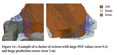
There are, however, some octrees for which the model would be misleading as the probability of the prediction is high (over 0.4, indicating a small standard error, usually under 2 m), but for which the prediction error is large (error over 2 m). These octrees were plotted in a 3D view to identify the causes for the model's inaccuracy. Two observations were made. First, some of these octrees are randomly distributed and isolated, meaning the surrounding octrees were well predicted. These octrees would have limited effects on the visual interpretation of the predictions. Second, some of these octrees are grouped in clusters, meaning an area of a stope is not well predicted. From a visual analysis, these clusters are located in parts of the stopes that behaved abnormally. In the Figure 14. example, the large UB seems to be a muckpile left in the stope and therefore reflects the quality of the data and not the model.

 

 

Limitations

The quality of the predictions can vary from stope to stope and is attributed to the data quality, such as fault position being wrong or the OB and UB being controlled by different parameters than those that the model considers as critical. Sometimes an individual wall is not well predicted but the rest of the stope is. Figure 15 gives an example of inaccurate predictions where OB is expected for an UB region and vice-versa. The probabilities also failed to highlight the possibility of large OB in the footwall. From discussions with mine personnel, OB was expected due to the presence of a nearby fault in the hangingwall. Poor ground conditions were expected, which would have caused the rock to break towards the fault. The different outcome indicates information about the fault and its influence was inaccurate in this instance, which can occur because part of the structural model is inferred. The random forest does, however, perform better than the PLS and LDA model for this example.

 

 

Discussion

The new proposed design approach enables the prediction of stope performance at an octree level. This means the location and magnitude of OB and UB are predicted, allowing the user to visualize the expected CMS in 3D and calculate volumes of OB and UB from it. This is a step change from current practice, which can only predict performance at individual stope surface scale without identifying the location of OB, while UB is ignored. Three separate multivariate statistical models were tested for predicting the projected distance of OB and UB. When choosing the best model, three criteria need to be considered: the classification of the octrees as OB or UB, the prediction error (how close is the prediction to the actual measure) and how the predictions compare to the actual CMS in a 3D view. It is important to validate the last criterion if the model is used in the stope design process to provide accurate information for engineers to make decisions.

The accuracy of each model at classifying the octrees is similar. The random forest model performs better than the other two models when looking at the statistical metrics (Table V). For the three cases, the model performed better at classifying UB than OB. Similar statistical trends were observed for the three models, but the random forest model performed better statistically and visually. The PLS model would lead the engineer to the right assessment 50% of the time compared to 75% of the time for the random forest when analysing stope face performance, which indicates a high success rate for the random forest model. The model would bring valuable insight to the engineers during the design, unlike anything before.

The PLS and random forest models take two different approaches to predicting stope performance. While PLS is a linear approach, random forest is a nonlinear approach and is better adapted for the complex interaction between blasting, the rock mass properties, the stope geometry, and stope performance. This is seen by the parameters' importance in the models (Table VI), which change according to the predictive model. The PLS model assigns more importance to the equivalent radius factor (ERF) parameter and this is seen in the predictions as the projected distance increases towards the middle of the faces. For the random forest model, the stope geometry and orientation are important parameters for making a prediction. Since the model generates useful predictions, the parameters' importance is used to interpret, to a certain degree, which parameters seem to influence the stope performance more. In this case, the blasting energy proxy, the stope geometry and orientation, and how the drifts cut the stope faces are probably the most important parameters for determining the stope performance, followed by the presence of faults.

 

 

Table VII presents the random forest model's performance at correctly classifying OB and UB according to the rounded projected distance. This allows the comparison of the model's OB and UB classification performance according to the projected distance that was measured with the post-mining CMS. The distance was rounded to the lowest unit, creating 10 classes. The model is less accurate in classifying octrees with small OB (0 to 1 m) as OB (61%) but performs very well for classifying octrees with a larger projected distance of OB or UB (over 80%).

This indicates that the locations where large OB and UB occur have certain characteristics quantified by the parameters that indicate that OB and UB will occur in these locations and will reliably identify these octrees as OB or UB. Therefore, given the selection of parameters used, critical portions of the stope are efficiently classified as OB or UB. These locations are key for optimizing the design. These numbers also reflect the quality parameters selected.

In addition, probabilities are generated for the predictions with random forest which enables the user to develop a probabilistic approach to stope design. This means different geometry of the mined shape can be built. The engineer can build a mean and worst-case geometry for assessing the expected stope performance. Therefore, the random forest model is the recommended statistical multivariate model for generating predictions based on the models presented in this paper.

Testing of the random forest model showed that the predictions are quickly generated (less than five minutes). The process can be interactive, where the engineer generates a prediction and, based on the results, modifies certain parameters to optimize stope performance and obtain a new set of predictions. This can be done for one stope or multiple stopes at once if a certain area or period of mining needs to be analysed. The predictive model is flexible and can be generated for different sectors, types of stope, and be updated over time. Stopes can be added to the model or removed if they are outdated, making sure the stopes in the model are relevant to the stopes being predicted.

This new stope design approach started with collecting mine site data and quantifying parameters at an octree resolution. Through multivariate analysis, an accurate understanding of the stope performance was established and the critical parameters were identified (McFadyen et al., 2023). Stope performance was predicted at an octree's resolution, as demonstrated in this paper, using a multivariate model. The good quality results of this first attempt at a complete prediction of the stope geometry using a random forest predictive model show the power and possibilities of using multivariate analysis to predict stope performance and spatially visualize what the CMS shape could look like. The standard error is used to create probability shells. As further work is done to refine and define input parameters at an octree resolution, the model can be refined, improving the predictions of the stope geometry.

The predictions could be implemented at the two main stages in the stope design process. There is the long-term design where the design geometry is established and the short-term design, closer to the mining date, where the operational parameters such as the drill rings are established. The selected parameters for the model would vary.

 

Summary and conclusion

Multivariate statistical models were built using parameters quantified at an octree resolution to predict stope performance; more precisely, predicting the location and magnitude of overbreak (OB) and underbreak (UB) at each point along the design surface. This novel approach significantly increases the capability of mine sites to optimize stope performance at the design stage due to the resolution of the analysis (per octree) and the wide range of parameters considered which are known to impact stope performance. Of the three tested statistical models (PLS, LDA, and random forest), the random forest approach was the most suitable for predicting stope performance at an octree resolution, correctly classifying octrees as OB or UB 67% of the time with the predictions being 65% of the time within 1 m of the actual surface in that location. From the 3D view analysis, 75% of the stope faces (hangingwall, footwall, sidewalls and, crown) that were predicted would have led an engineer to an accurate expectation of the face OB and UB in terms of location and magnitude. These predicted results can be included in the stope design step for optimizing stope performance.

This methodology results in an accurate and site-specific predictive model which is available at the stope design stage. The multivariate approach enables the user to consider multiple critical parameters and their complex relationship to understand the effect on OB and UB locally, and to predict stope performance and CMS shape. This empirical approach is easily applied at any mine site, allowing a complete and good quality database of the sites' stopes to be built at the same time, making it quick and easy to predict stope performance by simply importing a design geometry or drill-ring design and running the model.

 

Acknowledgement

The authors thank the sponsors for permission to use their data in this paper. This research would not be possible without the six industry sponsors of the project, the Minerals Research Institute of Western Australia (MRIWA), and the ongoing collaboration from mine site personnel. The sponsors were: BHP (Olympic Dam), Glencore (Mount Isa), IAMGOLD Corporation (Westwood), MMG Limited (Dugald River), OZ Minerals (Prominent Hill), and Newmont (Tanami). We gratefully acknowledge both corporate and individual support.

 

References

Adökö, A.C., Saadaari, F., Mirekü-Gyimah, D., and Imashev, A. 2022. A feasibility study on the implementation of neural network classifiers for open stope design. Geotechnical and Geological Engineering, vol. 40. pp. 677-696. https://doi.org/10.1007/s10706-021-01915-8        [ Links ]

Breiman, L. 2001. Random forest. Machine Learning, vol. 45. pp. 5-32. https://doi.org/10.1023/A:1010933404324        [ Links ]

Clark, L. 1998. Minimizing dilution in open stope mining with a focus on stope design and narrow vein longhole blasting. Master's thesis, University of British Columbia, Vancouver. 357 pp. https://open.library.ubc.ca/soa/cIRcle/collections/ubctheses/831/items/1.0081111        [ Links ]

Clark, L. and Pakalnis, R. 1997. An empirical design approach for estimating unplanned dilution from open stope hangingwalls and footwalls. Proceedings of the 99th CIM-AGM, Vancouve. CIM, Montreal.         [ Links ]

Fisher, R.A. 1936. The use of multiple measurements in taxonomie problems. Annals of Eugenics, vol. 7, no. 2. pp. 179-188. https://doi.org/10.1111/j.1469-1809.1936.tb02137.x        [ Links ]

Guido, S. and Grenon, M. 2018. Contributions to geomechanical stope optimization at the Goldcorp Eleonore Mine using statistical analysis. Proceedings of the 10th Asian Rock Mechanics Symposium. Singapore. Society for Rock Mechanics & Engineering Geology, Singapore. 12 pp.         [ Links ]

Guido, S., Grenon, M., and Germain, P. 2017. Stope performance assessment at the Goldcorp Eleonoe mine using bivariate analysis. Proceedings of AfriRock 2017: Rock Mechanics for Africa, Cape Town. International Society of Rock Mechanics. pp. 1107-1124.         [ Links ]

Hassell, R., Villaescusa, E., de Vries, R., and Player, J.R. 2015. Stope blast vibration analysis at Dugald River underground mine. Proceedings of the 11th International Symposium on Rock Fragmentation by Blasting, Sydney. Australasian Institute of Mining and Metallurgy, Melbourne. 16 pp.         [ Links ]

Hastie, T., Tibshirani, R., and Friedman, J. 2017. The Elements of Statistical Learning: Data Mining, Inference, and Prediction. 2nd edn. Springer, New York. 764 pp. https://doi.org/10.1007/978-0-387-84858-7        [ Links ]

Hughes, R. 2011. Factors influencing overbreak in narrow vein longitudinal retreat mining. Master's thesis, McGill University. 143 pp.         [ Links ]

Liland, K.H., Mevik, B.-H., Wehrens, R., and Hiemstra, P. 2020. pls: Partial Least Squares and Principal Component Regression. R package version 2.7-3. The Comprehensive R Archive Network. https://cran.r-project.org/        [ Links ]

Mathews, K.E., Hoek, E., Wyllie, D.C., and Stewart, S.B.V. 1981. Prediction of stable excavation spans for mining at depth below 1,000 m in hard rock mines. Report 802-1571. CANMET. Ottawa, Canada.         [ Links ]

Matthews, B.W. 1975. Comparison of the predicted and observed secondary structure of t4 phage lysozyme. Biochimica et Biophysica Acta-Protein Structure, vol. 405, no. 2, pp. 442-451.         [ Links ]

McCulloch, WS. and Pitts, W. 1943. A logical calculus of ideas immanent in nervous activity. Bulletin of Mathematical Biophysics, vol. 5, pp. 115-133. https://doi.org/10.1007/BF02478259        [ Links ]

McFadyen, B. 2020. Determination de facteurs contrölant la stabilité des chantiers souterrains pour une mine sujette ä la sismicité. Master's thesis, Université Laval, Canada. 146 pp. https://corpus.ulaval.ca/entities/publication/5b4c3a9b-9179-4821-ae3b-3939c84c233e        [ Links ]

McFadyen, B., Woodward, K R , Potvin, Y., and Grenon, M. 2020. A new stope reconciliation approach. UMT 2020: Proceedings of the Second International Conference on Underground Mining Technology. Wesseloo, J. (ed.). Australasian Institute of Mining and Metallurgy, Melbourne. pp. 335-350. https://doi.org/10.36487/ACG_repo/2035_17        [ Links ]

McFadyen, B., Woodward, K., and Potvin, Y. 2021. Open stope design; beyond the Stability Graph. Proceedings of the Underground Operators Conference 2021. Australasian Institute of Mining and Metallurgy, Melbourne. 13 pp.         [ Links ]

McFadyen, B., Grenon, M., Woodward, K., and Potvin, Y. 2023. Assessing stope performance using georeferenced octrees and multivariate analysis. Mining Technology, vol. 132, no. 2. pp. 132-152. https://doi.org/10.1080/25726668.2023.2205080        [ Links ]

Miller, F., Potvin, Y., and Jacob, D. 1992. Laser measurement of open stope dilution. CIM Bulletin, vol. 85. pp. 96-102.         [ Links ]

Nickson, S.D. 1992. Cable support guidelines for underground hard rock mine operations. Master's thesis. University of British Columbia. 223 pp. https://open.library.ubc.ca/media/stream/pdf/831/1.0081080/2        [ Links ]

Potvin, Y. 1988. Empirical open stope design in Canada. PhD thesis, University of British Columbia. 372 pp. https://open.library.ubc.ca/soa/cIRcle/collections/ubctheses/831/items/1.0081130        [ Links ]

Potvin, Y., Grant, D., Mungur, G., Wesseloo, J., and Kim, Y. 2016. Practical stope reconciliation in large-scale operations Part 2, Olympic Dam, South Australia. Proceedings of the Seventh International Conference & Exhibition on Mass Mining, Sydney. Australasian Institute of Mining and Metallurgy, Melbourne. pp. 501-509.         [ Links ]

Potvin, Y. and Hadjigeorgiou, J. 2001. The stability graph method for open-stope design. Underground Mining Methods, Engineering Fundamentals and International Case Studies. Hustrulid, WA. and Bullock, R.L. (eds). Society for Mining, Metallurgy & Exploration, Littleton, CO. pp. 513-520        [ Links ]

Potvin, Y., Woodward, K., McFadyen, B., Thin, I., and Grant, D. 2020. Benchmarking of stope design and reconciliation practices. UMT 2020: Proceedings of the Second International Conference on Underground Mining Technology, Australian Centre for Geomechanics, Perth. Wesseloo, J. (ed.). Australasian Institute of Mining and Metallurgy, Melbourne. pp. 299-308, https://doi.org/10.36487/ACG_repo/2035_14        [ Links ]

Qi, C., Fourie, A., Du, X., and Tang, X. 2018. Prediction of open stope hangingwall stability using random forests. Natural Hazards, vol. 92. pp. 1179-1197. https://doi.org/10.1007/s11069-018-3246-7        [ Links ]

R Core Team. 2021. R: A language and environment for statistical computing. Astria: R Foundation for Statistical Computing, Vienna. https://www.R-project.org/        [ Links ]

Venables, W.N. and Ripley, B.D. 2002. Modern Applied Statistics with S. 4th edn. Springer, New York. 498 pp. https://doi.org/10.1007/978-0-387-21706-2        [ Links ]

Wang, J. 2004. Influence of stress, undercutting, blasting and time on open stope stability and dilution. PhD thesis, University of Saskatchewan. 303 pp. https://harvest.usask.ca/handle/10388/etd-11032004-094152        [ Links ]

Wold, H. 1966. Estimation of principal components and related models by iterative least squares. Multivariate Analysis. Krishnajah, P.R. (ed.). Academic Press, New York. pp. 391-420.         [ Links ]

Woodward, K., McFadyen, B., Potvin, Y., and Wesseloo, J. 2019. Probabilistic stope design. MRIWA Project no. M489. Australian Centre for Geomechanics. Perth. 50 pp.         [ Links ]

Wright, M.N. and Ziegler, A. 2017. ranger: A fast implementation of random forests for high dimensional data in C++ and R. Journal of Statistical Software, vol. 77, no. 1. pp. 1-17. https://doi.org/10.18637/jss.v077.i01        [ Links ]

 

 

Correspondence:
M. Grenon
Email: Martin.Grenon@gmn.ulaval.ca

Received: 2 May 2023
Revised: 25 May 2023
Accepted: 21 Jun. 2023
Published: June 2023