PROFESSIONAL TECHINICAL AND SCIENTIFIC PAPERS

 

A critical comparison of interpolation techniques for digital terrain modelling in mining

 

 

M.A. Razas^I; A. Hassan^II; M.U. Khan^I; M.Z. Emach^I; S.A. Saki^I

^IUniversity of Engineering & Technology, Lahore. ORCID: M.A. Raza: http://orcid.org/0000-0001-5373-8795; M.U. Khan: http://orcid.org/0000-0002-6260-6679;M.Z. Emad: http://orcid.org/0000-0001-8537-8026
^IIUniversity' de Liege, Belgium

Correspondence

 

 

---

SYNOPSIS

Digital modelling of a surface is crucial for Earth science and mining applications for many reasons. These days, high-tech digital representations are used to produce a high-fidelity topographic surface in the form of a digital terrain model (DTM). DTMs are created from 2D data-points collected by a variety of techniques such as traditional ground surveying, image processing, LiDAR, radar, and global positioning systems. At the points for which data is not available, the heights need to be interpolated or extrapolated from the points with measured elevations. There are several interpolation/extrapolation techniques available, which may be categorized based on criteria such as area size, accuracy or exactness of the surface, smoothness, continuity, and preciseness. In this paper we examine these DTM production methods and highlight their distinctive characteristics. Real data from a mine site is used, as a case study, to create DTMs using various interpolation techniques in Surfer® software. The significant variation in the resulting DTMs demonstrates that developing a DTM is not straightforward and it is important to choose the method carefully because the outcomes depend on the interpolation techniques used. In mining instances, where volume estimations are based on the produced DTM, this can have a significant impact. For our data-set, the natural neighbour interpolation method made the best predictions (R² = 0.969, β = 0.98, P < 0.0001).

Keywords: digital terrain model, interpolation, topographic surface.

---

 

 

Introduction

Representation of the Earth's surface or terrain in an uncomplicated way and with high fidelity is crucial Earth scientists and engineers for many reasons. The representation of the Earth has evolved from simple paintings in ancient times to highly advanced digital representation in the form of digital terrain models (DTMs). A DTM is a representation of the topographic surface and is defined as the digital description of the terrain using a set of spot heights over a reference surface (Hirt, 2014). The concept of DTMs was first introduced during the late 1950s (Miller, 1958) and since then has come a long way. Photogrammetric techniques paved the way for producing DTMs (Thursston and Ball, 2007), which in turn have been extremely useful in geoscience applications since the 1950s and have become a major tool in geographical information processing (Weibel and Heller, 1991). DTMs are considered 2.5D models instead of fully 3D because they assign a unique height value to geodetic or planar coordinates, and thus topographic surfaces are usually shown as continuous surfaces or fields (Weibel and Heller, 1991; Hirt, 2014).

Along with DTMs, terms like digital surface models (DSMs) and digital elevation models (DEMs) are also commonly used, which should be distinguished from each other. A DSM is a depiction of a surface with all of its natural and built/artificial features such as vegetation and buildings, whereas a DTM is a bare earth surface. A DTM shows the development of a geodesic surface that augments a DEM and includes features of the natural terrain such as waterways and ridges. So a DEM can be created by interpolating a DTM but the reverse is not possible (GEODETICS, 2022). DEM, meanwhile, is a generic term that is used for a DTM as well as a DSM. It is synonymous with DTM if surface features like vegetation and building heights are removed during surveying, and if not, it is the same as DSM (Hirt, 2014; Maune, 2007). Irrespective of the terminology, all these terrain models are based on surface data-points.

 

DTM data sources

Data acquisition is a crucial task for creation of accurate map and terrain models. This has prompted the development of methods that provide maximum detail with high precision and accuracy. The usual techniques for data acquisition include traditional ground surveying, image processing (photogrammetry), LiDAR, radar- (radar interferometry), and global positioning systems (GPS) (Hirt, 2014).

Generally, traditional ground surveys have been the most common and cost-effective data-acquisition methods for limited areas and small projects and are more common for mining projects. Optical instruments such as theodolites, tachometers, and surveyor's levels have been utilized largely in the past; however, their use is decreasing because of their lower time efficiency and accuracy (Kennie and Petrie, 2010). Ground-based surveys are nowadays conducted with modern electronic equipment, which offers high-speed working and efficiency. The photogrammetric technique involves aerial or satellite images of the Earth's surface. These imaging techniques have benefitted from recent technological improvements and choosing between the two can be challenging. However, in general, the resolution of aerial images is higher than that of satellite images available for public use.

LiDAR (light detection and ranging) systems utilize a laser scanner, an inertial measurement unit (IMU), and a global positioning system (GPS) coupled with a computer to ensure that all the measurements are synchronous with respect to time. The procedure for LiDAR is such that an aircraft or helicopter flies above the area of interest and laser scan it from side to side. This results in a set of points recorded which contain the location and elevation information. The spatial density of these points is generally within one metre (Réjean, Pierre, and Mohamed, 2009). Radar interferometry is another method used for DTM data acquisition. This method can be used over land, sea, and ice surfaces. These radars use the microwave region of the electromagnetic spectrum, the same as SAR (synthetic aperture radar) systems. In principle, they are very similar to LiDAR in that they also utilize the features of back-reflected waves to determine surface features (Bamler, 1997). Wilson (2012) discusses the methods and data sources to generate DEMs using LiDAR and similar methods.

Recently, unmanned aerial vehicles (UAVs) and drones have become popular for topographic surveying and the creation of DTMs in mining and other fields. The success of these approaches hinges on their lower cost, flexibility, speed, and precision (Park and Choi, 2020; Yan, Zhou, and Li, 2012; Wajs, 2015). These devices use several downward-facing sensors and cameras to capture images during flight. The data is synchronized with a global information system (GIS) for accuracy. The gathered data is then processed using purpose-built modern software for DTM creation. In high-production open pit mining operations, such as strip mining, these techniques become especially useful as the volume computations can be done rapidly for accurate material excavation and overburden removal.

 

Sampling

From the 1970s onward, much research work was carried out on surface modelling and contouring from DEM and many interpolation techniques were proposed (Li, Zhu, and Gold, 2004). Methods such as different types of moving averages, height interpolation by finite element projective interpolation, kriging, and several triangulation methods were introduced. But with time it was realized that for a given topography, sampling is the critical factor (Li, Zhu, and Gold, 2004). As a result, attention shifted toward quality control and sampling methods.

Sampling has evolved into a whole new discipline and researchers have developed methods for the selection of suitable sampling techniques. Selective sampling, regular sampling patterns, and progressive and composite sampling are some of the popular photogrammetric sampling techniques. In selective sampling, commonly employed in field surveying, the points that are considered important are surveyed so as to have adequate coverage and required density. This method offers the advantage of high constancy with fewer points. The method is generally more useful for regions with major discontinuities and rugged terrain (Weibel and Heller, 1991). Regular sampling, also known as systematic sampling, as the name implies, uses a fixed distance between sampling points, which can be arranged as grids or profiles, square or rectangular. As the sampling interval is constant, it must be ensured that an adequate distance is selected in order to detect most of the discontinuities (Weibel and Heller, 1991; Li, Zhu, and Gold, 2004). It is a simple method that can be used in an automatic mode, but is restricted to fairly low and homogeneous terrains. In regions where discontinuities are more marked and the terrain is rugged, this might result in insufficient points to generate a high-fidelity terrain model (Weibel and Heller, 1991). In progressive sampling, a low-density grid is sampled initially, and wherever necessary a repetitive densification of the grid is performed; the whole area is surveyed until the required accuracy is achieved (Weibel and Heller, 1991, Li, Zhu, and Gold, 2004).

DTM data is judged by its distribution, density, and the accuracy with which it is measured (Li, Zhu, and Gold, 2004). Data can be distributed in various patterns but a particular pattern must fit the specific terrain being investigated. Density of sampled data is represented as either sampling interval or the number of points per unit area. Accuracy of the sampled data depends on the surveying method, quality of instrumentation, techniques used and the skill level of the surveyor. Data acquired in dynamic mode is likely to be less accurate than in static mode. Generally, it is considered that the field survey method is the most accurate, but this depends on the quality of the instrumentation used (Li, Zhu, and Gold, 2004).

 

Surface modelling

Surface modelling or surface reconstruction is the process by which the representation of terrain is obtained (Li, Zhu, and Gold, 2004). This reconstructed surface is the DTM surface that is generated from the original raw data and structured through a few popular approaches such as triangular irregular networks (TINs) and grid-based data structures (Li, Zhu, and Gold, 2004; Weibel and Heller, 1991).

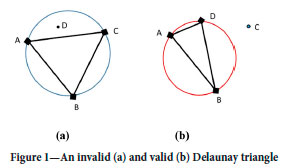
In TINs, the points or vertices are chosen and joined together in a series to form a network of triangles and therefore the surface is represented in the form of contiguous, non-overlapping triangles (ESRI, 2017). TINs have an advantage over grid-based models in their ability to describe the surface at different resolutions because in certain cases higher triangle resolution is required, such as for mountain peaks. (ET Spatial Technologies, 2017). TINs are also capable of working with any data pattern and can incorporate features like break lines (Li, Zhu, and Gold, 2004). Several methods have been developed to create these triangles but the most widely adopted is Delaunay triangulation, used by ArcGIS. Delaunay triangulation is based on the principle that a circle drawn through three nodes will not contain any other node This is known as the empty circumcircle principle (ESRI, 2017; ET Spatial Technologies, 2017; Li, Zhu, and Gold, 2004, as illustrated in Figure 1. The major advantage that this triangulation method offers over the others is that it produces as many equiangular triangles as possible and significantly reduces the chances of long, skinny triangles (ESRI, 2017;, ET Spatial Technologies, 2017). Moreover, there are certain interpolation techniques such as natural neighbour, which can only be applied to Delaunay-conforming triangles (ESRI, 2017). TIN is a frequently used vector data format for DEM and requires less computer memory than the gridded elevation models. However, because of the irregularity of the TIN, the organization, storage, and application of data are more complicated than that of the regular grid DEM (Liang and Wang 2020).

 

 

The other widely used approach is grid-based surface modelling where points are joined in the form of matrices, either regular squares or rectangles (Weibel and Heller, 1991;, Li, Zhu, and Gold, 2004). Handling of these matrices is simpler but a high point density is required to obtain a terrain of desired accuracy (Weibel and Heller, 1991). Grid-based modelling results in a series of contiguous bilinear surfaces (Li, Zhu, and Gold, 2004). Grid-based surface modelling is highly compatible with grid or progressive sampling techniques, and some software packages accept only gridded data (Li, Zhu, and Gold 2004).

 

Interpolation of data

In digital terrain modelling, interpolation serves the purpose of calculating elevations at the points for which data is not available from the points which have known elevations. There is a need to form the missing links between the points for which data is acquired to cover the unobserved part; the data that is estimated using interpolation to create DTMs. Interpolation is extremely important in terrain modelling processes such as quality control, surface reconstruction, accuracy assessment, terrain analysis, and applications (Li, Zhu, and Gold, 2004).

 

Visualization of DTMs

After collecting the data, and creating the surface and interpolation models, the DTM has to be visualized so that it can be understood in the best possible way. The approaches used include texture mapping, rendering, and animation (Li, Zhu, and Gold, 2004)). Technological advances have made DTM visualization relatively easy and multiple tools and software are available for presenting the data in 3D and creating a DTM. GIS is the most commonly used.

 

Applications of DTMs

DTMs have wide-scale uses in various disciplines of science and engineering such as mapping, remote sensing, civil engineering, mining engineering, geology, geomorphology, military engineering, land planning, and communications (Li, Zhu, and Gold, 2004;, Catlow; 1986, Petrie and Kennie, 1987). DTMs have made a significant contribution in the mining industry since the first time they were employed. Initial land surveys, reserve estimation, mine planning and, when the mining starts, setting up the equipment and the scheduling of mine machinery, all involve the use of DTMs. but the foremost application is in reserve estimation. A complete knowledge of the topographic surface of the region is necessary in defining the extent of the region and for large volume calculations. DTMs can also be used for highwall face and tunnel design and to calculate the volume of earthworks required for the completion of these tasks.

 

Interpolation techniques and mathematical models

Interpolation is an integral part of constructing a digital terrain model as it approximates data in the regions where none exists. After creating a grid (surface modelling) to represent a surface, we are left with plenty of nodes for which data is necessary and which is estimated using several interpolation techniques. This is even required for LiDAR although the point density is very high, but here it is intended to stick with the methods used for traditional field survey techniques and to interpolate the data for creating DTMs. The interpolation techniques that will be considered are IDW (inverse distance weighted), natural neighbours, kriging, and splines. Different criteria for classifying interpolation techniques are applied across the globe in diverse fields. Some of them are discussed below.

There are many ways in which interpolation techniques can be classified, such as based on area size, accuracy or exactness of the surface, smoothness, continuity, and preciseness. Several interpolation techniques have been developed by mathematicians and researchers and to date, even after much work, no technique is considered as the general best (Weibel and Heller, 1991).

An interpolator is either global or local if it is based on the scope or area of the field (Li, Zhu, and Gold, 2004; Gentile, Courbin, and Meylan, 2013). Global interpolators are those which use all of the measured points or the whole sampled region to estimate values for the unknown points, whereas local interpolators use a patch or some points close to the targeted value (Gentile, Courbin, and Meylan, 2013). Burrough et al. (2015) suggest that global interpolators are suitable for describing the general trend of terrain, while local interpolators are preferable for variations over patches and utilizing spatial relationships between the data. Based on the interpolated value, they are either exact, where the interpolated value for an already sampled point will be the same as the measured, or approximate, where the interpolated value differs from the known measured value (Gentile, Courbin, and Meylan,, 2013). In other words, exact interpolators result in DTM surfaces that pass through every sampled point while approximate interpolators follow a trend instead and may not necessarily pass through all the original points (Maguya, Junttila, and Kauranne, 2013). This is because of the fact that some methods incorporate certain smoothing functions just to smooth out the sharp changes that might be incorporated (Gentile, Courbin, and Meylan, 2013). All these interpolation techniques basically have a mathematical or statistical model designed to subsume different parameters which affect the interpolation results. Based on these models, interpolation techniques are either deterministic or stochastic. Stochastic or geostatistical methods are those that are capable of yielding the estimated value as well as the associated error whiledeterministic methods, on the other hand, do not include any assessment of the error which could be associated with the estimated value (Gentile, Courbin, and Meylan, 2013). Interpolation methods are concerned with finding out if the values are interrelated, i.e. correlation and dependency (Childs, 2004). This correlation is then used to measure the similarity index within an area, the level, strength, and nature of interdependence between the variables (Childs, 2004). This section focuses on the mathematical or statistical models of the above techniques.

Inverse distance weighting

Inverse distance weighting (IDW) is a local interpolation method that gives exact measurement values and utilizes a deterministic model. There are specific algorithms that can be used to achieve smoothness (Gentile, Courbin, and Meylan, 2013). IDW assumes that the values which are closer to the point to be interpolated will be somewhat similar to those which are further away. Based on this assumption that the nearest points will influence the results greatly, IDW uses them to assign values for unmeasured locations. IDW is an example of a deterministic method, therefore the results will be same even if interpolation is repeated several times. According to its mathematical model, IDW is represented by Equation [1].

where Z(s_o) is the value that needs to be estimated at location so, N is the number of samples chosen in a particular search distance, λ_i, is the weight assigned to each sampled point, and Z(s¡) is the known measured value at location s¡ (Erdogan, 2009, Jones et al., 2003). The equation that is developed for calculating weights involves an inverse relation with exponents (x) of distance (d) between the known value and the point to be predicted. Equation [2] is used to calculate the assigned weights, λ_i .

The exponent parameter x indicates the degree of influence of the surrounding points on the estimated value (Priyakant, Rao, and Singh, 2003). The weights sum to unity, showing that the method is unbiased (Gentile, Courbin, and Meylan, 2013). It is evident from Equations [1] and [2] that an increase in distance d will decrease the influence on the interpolated value (Burrough et al., 2015). It is also true that higher values of x will result in smaller weight values assigned for distant points, and lower values in larger weights (Erdogan, 2009, Aguilar et al., 2005). Therefore, the extreme values in the terrain will be sharper and it can be said that the parameter x controls the degree of smoothness in the IDW case. The value of x used typically varies between 1 and 4 with 2 the most commonly used, the reason why this technique is often referred to as inverse distance square (IDS) (Aguilar et al., 2005; Kravchenko and Bullock, 1999; Gentile, Courbin, and Meylan, 2013). Different x values and their impact on interpolation estimate quality have been studied by many researchers and it has been found that the power factor can be of great significance, or in some cases (Aguilar et al., 2005) may not affect the results very much.

The other very important factor associated with IDW is the minimum number of points to be taken into consideration (Kravchenko and Bullock, 1999; Gentile, Courbin, and Meylan, 2013) as more points result in increased smoothing (Gentile, Courbin, and Meylan, 2013). Although the choice of x and N is tricky, methods such as cross-validation and jackknifing can be used to select the most appropriate values for these two most important parameters (Tomczak, 1998). The size and shape of the search radius are also very important and should be chosen very carefully. If there is no observable directional influence on the weights of data, the shape of the search radius should preferably be a circle, and if otherwise, it should be adjusted likewise (ESRI, 2017). Size is also an indication of the degree of influence the distant point has on the location to be interpolated.

IDW is widely used because of its simplicity, lower computational time, and its ability to work with scattered data (Gentile, Courbin, and Meylan, 2013), but there are also some drawbacks associated with it. These are the selection of interpolation parameters, exact interpolation which refers to no smoothing, its deterministic nature as it doesn't possess the ability to incorporate errors, and above all, IDW is highly sensitive to outliers and clustered data which can result in biased results, because of which IDW interpolated surfaces consist of features such as peaks and dips (Gentile, Courbin, and Meylan, 2013). Although IDW itself is an exact interpolator, some algorithms have been developed to incorporate a smoothing factor and the equation can also be written as Equation [3] (Gentile, Courbin, and Meylan, 2013; Garnero and Godone, 2013). Typically, a value between 1 and 5 is taken for s and it reduces the influence of any one sample for interpolated value (Li, Liu, and Chen, 2011).

Splines

Splines are basically polynomials of degree k which are fitted between each point to define the surface completely (Gentile, Courbin, and Meylan, 2013, Li and Heap, 2011). The places where two separate polynomials meet are called 'knots' and these knots can have a huge impact on the interpolation results (Li and Heap, 2011). The challenge is always to gradually smooth out the surface at these knots, and the method revolves around making the polynomial function, its first-, and in some cases, the second-order derivative, continuous at these arbitrarily chosen knots (Gentile, Courbin, and Meylan, 2013). However, this piecewise polynomial reference is different from that in raster interpolation where it refers to radial basis functions (Skytt, Barrowclough, and Dokken, 2015), which will be the area of focus here.

Splines is the method that estimates the values using mathematical functions which smooth the surface and minimize the curvature of the surface (Childs, 2004). Splines have many variates and they produce surfaces which pass through all the sampled points and smooth the rest of it (Childs, 2004; Garnero and Godone, 2013). It is often referred to as a bending sheet (Childs, 2004) which is shaped to pass through all the sampled points and results in a smooth surface. Splines are global; they result in approximately estimated values and the model used is deterministic (Gentile, Courbin, and Meylan, 2013).

Splines have a basic form similar to IDW, in which weights are assigned according to the distance between known and unknown points (Garnero and Godone, 2013) as given by Equation [4].

where Φ(τ) represents the interpolation function and r shows the Euclidean distance between the known point si and the unknown point s_o which is represented as || s_i - s_o (Garnero and Godone, 2013). Although this is considered as standard, other types of distance function can also be utilized (Gentile, Courbin, and Meylan, 2013). The weights must be assigned in a manner such that the function chosen gives the exact measured value as this type of interpolation is supposed to be passing through all the known points (Garnero and Godone, 2013). This leads to n number of equations with n number of unknowns, which can be worked to acquire a unique solution (Garnero and Godone, 2013; ESRI, 2017). There are many spline functions that have been developed to improve the method further and make it adjustable for given conditions (Gentile, Courbin, and Meylan, 2013; Garnero and Godone, 2013).

In the above-stated mathematical expressions r is the Euclidean distance, σ is the tension parameter, E₁ is the exponential integral function, C_E is defined as the Eulero constant which has a value of 0.577215, and K₀ is termed the modified Bessel function (Gentile, Courbin, and Meylan, 2013). The tension parameter, σ, controls the smoothness of a function. The higher its value the better the smoothing, which can have adverse effects in a sense that the depiction of the data may not show the actual variation of the data (ESRI, 2017). This, however, is not true for the inverse multiquadratic method where the reverse is considered true (ESRI, 2017; Garnero and Godone, 2013). Keeping in view the challenge at hand of choosing an appropriate value for the smoothing factor, the same techniques of cross-validation and jack-knifing or trial and error are used. In ArcGIS, these functions are listed under radial basis functions, and a function can also be selected using cross-validation (ESRI, 2017). Many consider multi-quadratic to be the best function (Yang et al., 2004).

Splines offer some advantages over the other techniques in that the roughness of the terrain can be smoothed out efficiently and it is also capable of capturing broad and detailed features (Gentile, Courbin, and Meylan, 2013). The availability of many functions makes this method somewhat more flexible and adjustable to the data. This method works best for the terrains which have gentle slope variation and where the changes occur gradually over considerable horizontal distances (ESRI, 2017). It is also suitable for handling large data-sets (ESRI, 2017). A feature of this method that it can under- and over-estimate the given data for unknown points to make it a better fit for hills and smooth slopes. Splines can also be used along with other interpolation techniques to smooth an already created surface (Erdogan, 2009). Although splines outweigh other techniques in many respects, they do have their fair share of disadvantages. These include considerable variations in elevation within a short horizontal distance (ESRI, 2017), inability to give an account of errors because of their deterministic nature (Gentile, Courbin, and Meylan, 2013), empirical choice of the function and parameters selected (Gentile, Courbin, and Meylan, 2013), and their handling of clustered and isolated data swiftly (Gentile, Courbin, and Meylan, 2013). Furthermore, overall smoothing may still be too high (Gentile, Courbin, and Meylan, 2013) if the chosen values of parameters are not optimal.

Kriging

Kriging is an extensively used method (Meyer, 2004) that is favoured by many authors. Bailey (1994, p. 32) maintains that 'there is an argument for kriging to be adopted as a basic method of surface interpolation in geographic information systems (GIS) as opposed to the standard deterministic tessellation techniques that currently prevail and which can produce artificially smoothed surfaces'.

Kriging, unlike the other methods under discussion, is a family of geostatistical or stochastic methods (Gentile, Courbin, and Meylan, 2013; ESRI, 2017). Kriging tries to identify the spatial correlation between the data, in order to come to a better conclusion. This suggests that all the points around an unknown point may not necessarily influence it in the same manner. Therefore, this correlation is modelled as a function of the distance (Burrough et al., 2015). The value at any location is assumed to incorporate a certain component of the trend and a random variable following a special distribution (Clark, 1979).

Kriging is a method in which the value at an unknown point is estimated in two steps, i.e., calculating weights and then estimating the value. Determination of weights utilizes a function named the semivariogram y(h) (sometimes referred to as just variogram), and the process as variogram modelling, and is represented by Equation [5] (Clark, 1979), where 'n denotes the number of paired samples.

Variogram modelling is completed by constructing an experimental variogram' y^(h), and then fitting an 'authorized variogram' y(h), model against it (Gentile, Courbin, and Meylan, 2013). An experimental variogram (sometimes referred to as an empirical variogram) is subjected to the conditions and is calculated from the sample data rather than being theoretical (Clark, 1979). An authorized variogram, on the other hand, is any one of a few standard variogram models that have been developed theoretically (Gentile, Courbin, and Meylan, 2013; Clark, 1979). Semivariograms enable understanding the trend in data to further use it for defining two very important features - sill and range.

Kriging has many forms but Equation [6] can be considered the basis for all of them (Li and Heap, 2011). Here, μ is the stationary mean which is supposed to be constant over the whole domain and is calculated as the average of the data (Li and Heap, 2011). λ_i is the kriging weight, n denotes the number of known points used for the estimation of the unknown in a particular search window, and μ(so) is the mean of the samples within the search window (Li and Heap, 2011).

Among all the variants, ordinary kriging (OK) is the most widely used (Gentile, Courbin, and Meylan, 2013). Although many kriging methods are approximate, OK is an exact method and estimates the values locally (Gentile, Courbin, and Meylan, 2013). OK, based on its geostatistical properties, assumes the model as Equation [7].

where, μ is the constant because of the intrinsic stationarity, also known as a deterministic trend (Erdogan, 2009), but is unknown (Gentile, Courbin, and Meylan, 2013; ESRI, 2017), while ε(s) is a random quantity drawn from the probability distribution (Gentile, Courbin, and Meylan, 2013), ε(s)) is also called auto-correlated errors (Erdogan, 2009).

Kriging is sometimes referred to as BLUE (best linear unbiased estimator) (Gentile, Courbin, and Meylan, 2013). Kriging is the best method if there is a directional bias or spatial autocorrelation is present in the data (Childs, 2004). In kriging, unlike IDW, the estimated values can be greater than the sample values and the surface does not necessarily pass through all those sample points (Childs, 2004). Kriging is also capable of giving a quantifiable account of interpolation errors in kriging variance (Gentile, Courbin, and Meylan, 2013). Although kriging is highly favourable in plenty of conditions, it is an overall complex method which requires extreme care when spatial correlation structures are being modelled (Gentile, Courbin, and Meylan, 2013).

 

Comparison of interpolation techniques

Methodology

For a comparison of interpolation techniques, we used a real data-set from a large mining site. The data was collected using traditional and GPS-based surveying techniques. Using this data, several topographic surfaces were created using SURFER^® 9 utilizing various interpolation techniques.

SURFER^® 9 has multiple built-in interpolation techniques that make it easier to create surfaces using one method with a simple one-click operation, which makes it possible to handle and tinker with the methods under consideration.

The data

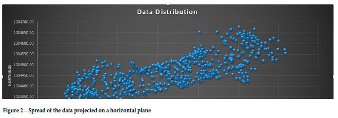
The raw data used for this analysis is presented in Figure 2. The points show little scatter and are confined in a positively sloping trend within a bigger arbitrary rectangular region roughly 500 χ 500 m in areal extent. We used this data to create a rectangular region using extrapolation. This will help in understanding the differences encountered while extrapolating the surface for the rectangular region using these points. Although the differences in elevations are not enormous, there are drops and rises in elevations within the data, with the difference between the maximum and the minimum elevation being around 30 m, which will help in identifying the key features related to each method.

Keeping in view the distribution of the data in Figure 2, the interpolated and the extrapolated regions can be analysed separately. Although extrapolated regions cannot be trusted for their accuracy because of data scarcity, they will help in understanding the key features of these techniques.

The inverse distance weighted to power (IDW) technique is worked by using the values 1, 2, and 4 for power parameter x. It is alredy understood that x refers to the weight that is to be given to the near and far points.

 

Results and discussion

The surfaces created using various interpolation techniques are presented in this section.

Interpolation using inverse distance weighting

The surfaces created using inverse distance weighting with power factors (x) of 1, 2, and 3 are presented in Figure 3. The parameter x controls the smoothing (Gentile, Courbin, and Meylan, 2013) and this is clearly visible in the interpolated region. The created surface is smoother where the degree of roughness increases with the power factor x. It can also be seen that with increasing values of x, sharp features such as pits become evident within the same region.

 

 

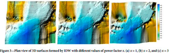
Moving towards the extrapolation region, the degree of smoothness behaves differently to that in the interpolated regions. This is due to the fact that IDW, with higher power values, assigns lower weights to the more distant points. Therefore, as the data becomes more distant, the surface starts to behave smoothly even for sharp changes in elevation. This observation is consistent with both sides of the sampled data.

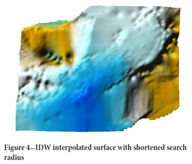
Another important parameter involved in IDW is the search radius, which in this case seems to have little effect on the generated surface, due primarily to the fact that the data is abundant for the region where it exists. However, if the search radius is too low, this can have an impact on the extrapolated surface such that the results may not be obtained for regions such as corners that might become offshore to a certain search radius limit. One such example is shown in Figure 4, where the power factor is kept as 2 while the search radius is taken as 150 yards instead of 342 for Figure 3 .

 

 

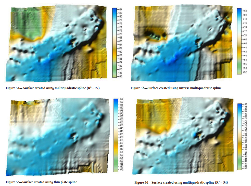
Interpolation using splines

Compared to IDW, splines show inconsistent behaviour between the different variants such as multiquadratic, inverse multiquadratic, and thin plate splines as shown in Figure 5. SURFER* 9 does not provide the option of using splines with tensions and completely regularized splines. This inconsistent behaviour culminates in the extrapolated region where there are large differences in elevation within a very short horizontal distance. In the interpolated region, however, the three kernel functions performed similarly.

A key feature associated with splines is their ability to over- and under-estimate the sampled points for an unknown point. The minimum and maximum elevation values among all the data-points are 450.02 and 483.33 yards respectively. Thin plate splines have been estimated as less as 375 yards and as high as 495, which is the greatest among the three variants utilized. The multiquadratic function also exhibited the same feature but only to a small extent, which seems more practical compared to thin plate splines where

the difference is too great to be considered practical, especially in the extrapolated region. It needs to be noted, however, that inverse multiquadratic did not exhibit the same feature. The multiquadratic function tested for twice the initial value of R², i.e. R² = 54 (Figure 5d) yielded minimum and maximum values of 436 and 490 respectively, compared with 446 and 484 for R2 = 27 (Figure 5a).

Interpolation using kriging

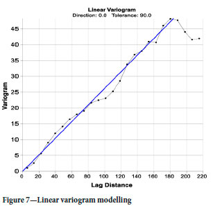
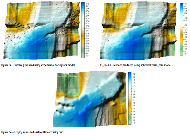
In interpolating with kriging, the most important factor to consider is the selection of an appropriate variogram model. Kravchenko and Bullock (1999) observed better soil parameter estimates with kriging and noted that kriging produced more accurate estimates compared to IDW when the variogram and number of neighbouring points were selected carefully. With the given set of points, the linear model proved to be the best fit while others (exponential and spherical) failed to predict the trend completely. Figures 6a and 6b represent the modelled surfaces using a spherical and an exponential variogram respectively. Kriging produced a smoother surface with slight underestimation of the interpolated values. Even in the extrapolated region, surfaces are smoother than those with splines, and to some extent with IDW. The smoothness of the surface in this case for kriging is due to the fact that the datapoints are closely spaced and kriging treats the clustered location more like a single point. These points are sampled because of the changes in their elevations, which kriging fails to pinpoint clearly. Figure 6c shows a surface produced using the best fit variogram linear model. The linear model is shown in Figure 7.

 

 

Interpolation using natural neighbour technique

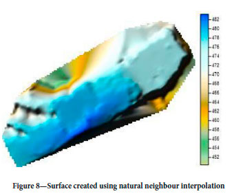
Natural neighbour interpolation (NNI) performs fairly well apart from in the extrapolated region where there are no results at all. Figure 8 represents the surface created utilizing NNI, which is smooth compared with IDW and splines. NNI was also capable of estimating small changes in elevation and still producing a smoother surface. As expected, it did not over- or underestimate the data at all. Because of the simple procedure, the computational time for this method was much less. One of the possible reasons for the surface being smooth may be the small horizontal distance between the data-points. NNI handles the scattered data well because it creates polygons and when data-points are too close to each other, there might be some numerical instability and errors in rounding off.

 

 

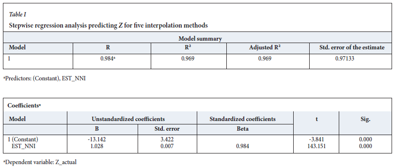
Predicting best fit through regression modelling

To determine which interpolation method predicted/estimated the original heights/elevations (Z values) the best, we conducted a stepwise regression analysis by including the Z value estimates using inverse distance weighting (EST_IDW1, EST_IDW2, EST_IDW3 with weights 1, 2, and 3 respectively), kriging (EST_KRG), and natural neighbour (EST_NNI). The analysis (Table I) indicated EST_NNI as the best predictor for the original Z values (R² = 0.969, β = 0.98, P < 0.0001). This may be because of the fact that the data- set was large and closely spaced enough to provide the best estimate. All the interpolation methods produced very close estimates of the Z values.

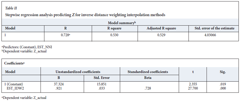
As inverse distance weighting is a popular interpolation method for DTMs created for mining purposes because of its simplicity to comprehend and use, we compared the three inverse distance weighted estimates (EST_IDW1, EST_IDW2, and EST_IDW3). Among these, the inverse distance squared method (EST_IDW2) proved to be the best estimator for the given set of data (R² = 0.530, β = 0.728, P < 0.0001) (Table II).

 

Conclusions

An overview of the common interpolation techniques used for creating digital terrain models (DTMs) in mining was presented. Asample data-set from an actual mine site was interpolated and extrapolated using inverse distance weighting (IDW), splines, kriging, and natural neighbour techniques in Surfer* 9. The results showed that the creation of a DTM is not a straightforward exercise, and one must be careful in selecting the method, as the results vary based on the choice of interpolation method and the data-set. This can have a huge impact in mining situations where volume calculations are based on the DTM created. The selected method must also incorporate both data interpolation and extrapolation. Although the IDW methods are most commonly employed for DTM creations in mining, this study shows that the results are strongly influenced by the search radius and the power factor of IDW. In general, kriging and natural neighbour produced better results for extrapolation, as these techniques do not overestimate or underestimate the data-points. The selection of any method must take into account various interpolation techniques and then gauge their benefits before finalizing a specific interpolation method for DTM creation. For our data-set, the natural neighbour interpolation method produced the best estimates.

For future research, the authors plan to compare the findings with a high-resolution satellite image or through field visits for higher fidelity. This, along with detailed statistical analysis and simulations, will help further refine the technique. These findings should help field mining and exploration engineers to produce better resource and volume estimates.

 

References

Agüilar, F. J., Agüera, F., Agüilar, M.A., and Carvajal, F. 2005. Effects of terrain morphology, sampling density, and interpolation methods on grid DEM accuracy. Photogrammetric Engineering & Remote Sensing, vol. 71. pp. 805-816.         [ Links ]

Bailey, TC. 1994. A review of statistical spatial analysis in geographical information systems. Spatial Analysis and GIS. Fotheringham, S. and Rogerson. P, (eds). CRC Press. pp. 13-44.         [ Links ]

Bamler, R. 1997. Digital terrain models from radar interferometry. https://phowo.ifp.uni-stuttgart.de/publications/phowo97/bamler.pdf        [ Links ]

Böhling, G. 2007. Introduction to geostatistics. Open File Report no. 26. Kansas Geological Survey. 50 pp.         [ Links ]

Bürröügh, P.A., McDonnell, R., McDonnell, R.A. and Lloyd, CD. 2015. Principles of Geographical Information Systems. Oxford University Press.         [ Links ]

Catlöw, D. 1986. The multi-disciplinary applications of DEMs. Proceedings of Auto-Carto London. Volume 1. Hardware, Data Capture and Management Techniques. Blakemore, M. (ed.). pp. 447-454. https://cartogis.org/docs/proceedings/archive/auto-carto-london-vol-1/pdf/the-multi-disciplinary-applications-of-dbms.pdf        [ Links ]

Childs, C. 2004. Interpolating surfaces in ArcGIS spatial analyst. ArcUser, July-September 2004. pp. 32-35.         [ Links ]

Clark, I. 1979. Practical Geostatistics. Applied Science Publishers, London.         [ Links ]

Erdögan, S. 2009. A comparision of interpolation methods for producing digital elevation models at the field scale. Earth Surface Processes and Landforms, vol. 34. pp. 366-376.         [ Links ]

ESRI. 2017. ArcGIS Documentation. https://desktop.arcgis.com/en/documentation/        [ Links ]

ET Spatial Technologies. 2017. Triangulated irregular network http://www.ian-ko.com/resources/triangulated_irregular_network.htm        [ Links ]

Garnerö, G. and Gödöne, D. 2013. Comparisons between different interpolation techniques. Proceedings of the International Archives of the Photogrammetry, Remote Sensing and Spatial Information Sciences, vol. XL-5/W3. pp. 27-28. https://d-nb.info/1144994764/34        [ Links ]

Gentile, M., Cöürbin, F., and Meylan, G. 2013. Interpolating point spread function anisotropy. Astronomy & Astrophysics, vol. 549. A1. 20 pp. https://www.aanda.org/articles/aa/full_html/2013/01/aa19739-12/aa19739-12.html        [ Links ]

Geödetics. 2022. DEM, DSM & DTM: Digital elevation model - Why it's important https://geodetics.com/dem-dsm-dtm-digital-elevation-models/        [ Links ]

Hirt, C. 2014. Digital terrain models. Encyclopedia of Geodesy. Grafarend, E.W (ed.). Springer, Berlin, Heidelberg. https://ddfe.curtin.edu.au/gravitymodels/ERTM2160/pdf/Hirt2015_DigitalTerrainModels_Encylopedia_av.pdf        [ Links ]

Johnston, K., Ver Höef, J.M., Krivörüchkö, K., and Lucas, N. 2001. Using ArcGIS geostatistical analyst. Esri Press, Redlands, CA. https://downloads2.esri.com/support/documentation/ao_/Using_ArcGIS_Geostatistical_Analyst.pdf        [ Links ]

Jones, N.L., Davis, R.J., and Sabbah, W. 2003. A comparison of three-dimensional interpolation techniques for plume characterization. Groundwater, vol. 41. pp. 411-419.         [ Links ]

Kennie, T.J.M. and Petrie, G. 2010. Engineering Surveying Technology, Taylor & Francis.         [ Links ]

Kravchenkö, A. and Bullock, D.G. 1999. A comparative study of interpolation methods for mapping soil properties. Agronomy Journal, vol. 91. pp. 393-400.         [ Links ]

Krivörüchko, K. and Gotway, CA. 2004. Creating exposure maps using kriging. Public Health GIS News and Information, vol. 56. pp. 11-16.         [ Links ]

Li, D., Liu, Y., and Chen, Y. 2011. Computer and Computing Technologies in Agriculture IV: 4th IFIP TC12 Conference. CCTA 2010, Nanchang, China, October 22-25, 2010, Part II, Selected Papers, vol. 345. Springer.         [ Links ]

Li, J. and Heap, A.D. 2011. A review of comparative studies of spatial interpolation methods in environmental sciences: Performance and impact factors. Ecological Informatics, vol. 6. pp. 228-241.         [ Links ]

Li, Z., Zhu, Q., and Gold, C. 2004. Digital Terrain Modeling: Principles and Methodology, CRC Press.         [ Links ]

Liang, S. and Wang, J. 2020. Geometric processing and positioning techniques. Advanced Remote Sensing (2nd edn). Academic Press. pp. 59-105.         [ Links ]

Maguya, A.S., Junttila, V., and Kauranne, T. 2013. Adaptive algorithm for large scale dtm interpolation from lidar data for forestry applications in steep forested terrain. ISPRS Journal of Photogrammetry and Remote Sensing, vol. 85. pp. 74-83.         [ Links ]

Maune, D.F. 2007. Digital Elevation Model Technologies and Applications : The DEM Users Manual. American Society for Photogrammetry and Remote Sensing, Bethesda, MD.         [ Links ]

Meyer, TH. 2004. The discontinuous nature of kriging interpolation for digital terrain modeling. Cartography and Geographic Information Science, vol. 31. pp. 209-216.         [ Links ]

Miller, CL. 1958. The theory and application of the digital terrain model. MS thesis, Massachusetts Institute of Technology.         [ Links ]

Park, S. and Choi, Y. 2020. Applications of unmanned aerial vehicles in mining from exploration to reclamation: A review. Minerals, vol. 10. p. 663.         [ Links ]

Petrie, G. and Kennie, T. 1987. An introduction to terrain modeling: Applications and terminology. Terrain Modelling in Surveying and Civil Engineering: A Short Course. University of Glasgow.         [ Links ]

Priyakant, N.K.V., Rao, L., and Singh, A. 2003. Surface approximation of point data using different interpolation techniques-A GIS approach. http://www.geospatialworld.net/article/surface-approximation-of-point-data-using-different-interpolation-techniques-a-gis-approach/        [ Links ]

Réjean, S., Pierre, B., and Mohamed, R. 2009. Airborne LIDAR surveys - An economic technology for terrain data acquisition.: https://www.geospatialworld.net/article/airborne-lidar-surveys-an-economic-technology-for-terrain-data-acquisition/        [ Links ]

Skytt, V., Barrowclough, O., and Dokken, T. 2015. Locally refined spline surfaces for representation of terrain data. Computers & Graphics, vol. 49. pp. 58-68.         [ Links ]

Thursston, J. and Ball, M. 2007. What is the role of the digital terrain model (DTM) today? http://sensorsandsystems.com/what-is-the-role-of-the-digital-terrain-model-dtm-today/        [ Links ]

Tomczak, M. 1998. Spatial interpolation and its uncertainty using automated anisotropic inverse distance weighting (IDW)-cross-validation/jackknife approach. Journal of Geographic Information and Decision Analysis, vol. 2. pp. 18-30.         [ Links ]

Wajs, J. 2015. Research on surveying technology applied for DTM modelling and volume computation in open pit mines. Mining Science, vol. 22. pp. 75-83.         [ Links ]

Weibel, R. and Heller, M. 1991. Digital terrain modeling. Geographical Information Systems: Principles and Applications. Maguire, D.J., Goodchild, M.F., and Rhind, D.W. (eds). Longman, London.         [ Links ]

Wilson, J.P.J.G. 2012. Digital terrain modeling. Geomorphology, vol. 137. pp. 107-121.         [ Links ]

Yan, X.M., Zhou, Z.L., and Li, X.B. 2012. Three-dimensional visual modeling technology and application of open pit mining boundary. Advanced Materials Research. Trans Tech, Stafa-Zurich, Switzerland. pp. 790-793.         [ Links ]

Yang, C.-S., Kao, S.-P., Lee, F.-B., and Hung, P.-S. 2004. Twelve different interpolation methods: A case study of Surfer 8.0. Proceedings of the XXth ISPRS Congress. International Society for Photogrammetry and Remote Sensing, Hannover, Germany. pp. 778-785.         [ Links ]

 

 

Correspondence:
M.U. Khan
Email: usman@uet.edu.pk

Received: 16 Aug. 2022
Revised: 16 Nov. 2022
Accepted: 18 Nov. 2022
Published: February 2023