PROFESSIONAL TECHNICAL AND SCIENTIFIC PAPERS

 

Real-time underground route identification and route progress using simple on-board sensing and processing

 

 

R.F. Meeser; N. Theron

University of Pretoria, Pretoria, South Africa. ORCID: R.F. Meeser: http://orcid.org/0000-0001-5546-883X

Correspondence

 

 

---

SYNOPSIS

The global emphasis on conserving energy resources has led to the adoption of hybrid power systems in vehicles. Optimally applied, hybrid systems can save up to 40% on fuel costs. To optimally manage a hybrid vehicle's energy flow it is necessary to know, in real time, all the energy requirements to complete a given route. The energy consumption depends mainly on the vehicle mass, speed profile, and route topography. Of these, the topographic profile is the one factor that is only route-dependent and not influenced by the vehicle or driving styles. The heading vs. distance profile is also an example of a route characteristic not influenced by the vehicle or driving style. In this study the topographic and heading profiles are used to identify routes, and are easily measured by means of digital barometric pressure and compass sensors. Correlations between the current route and previously travelled/stored routes are performed based on their topographic and heading profiles in a point-by-point manner. Above-ground tests were first performed using a road vehicle and six routes to evaluate the system. The system consistently and correctly identified a 20 km route within the first 4 km. It also proved to function correctly in underground tests through the implementation of an instrumented hand-held surveyor's wheel. This system finds direct practical application in optimizing the energy management of an underground hybrid locomotive used by the mining industry in South Africa, but can also be of benefit in applications where route identification is required and using GPS is not feasible.

Keywords: real-time route identification, underground navigation, topographic profile.

---

 

 

Introduction

Recently an increasing emphasis has been placed on improving vehicle efficiency and reducing waste in all forms (Taghavipour et al., 2016). One such improvement is the use of hybrid drivetrains in vehicles. Many hybrid electric vehicles (HEVs) comprise a combination of a fossil fuel internal combustion engine (ICE), electric motor (EM), electric motor driver (power electronics that control the power to and from the electric motor), energy storage systems (ESSs), inverters (to facilitate the energy flow), and a vehicle control system to manage all of these. Hybrid vehicles are equipped with sophisticated control strategies that are applied to achieve higher efficiencies than normal ICE-driven vehicles by allowing the use of the electrical systems to store or recover energy that would otherwise be wasted as well as enabling the ICE to operate in a more efficient region of its operating range (Huang et al., 2017). When correctly applyied, hybrid technology can decrease fuel consumption by up to 40% (Tie and Tan, 2013). The vehicle that this project focuses on is an underground hybrid electric locomotive that is used in the mining sector in South Africa. The locomotive has a 30 kVA tier 4 diesel generator set that is used to charge a 460 V, 160 Ah lithium iron phosphate (LiFePo4) battery pack. The battery pack provides the electrical energy that is used to power the locomotive's two 17 kW direct current (DC) motors, which in turn are connected to the wheels via a chain drive (CMTi Group, 2021).

Successful optimization of the energy system of an HEV relies on knowing not only the current state of the onboard energy systems, including fuel level, battery state of charge etc., but also the future demands that the locomotive will encounter on its route. These demands depend on variables such as the vehicle, drivetrain, route speed profile, route topography, and vehicle mass, all as a function of the route's distance to completion. The topography of a route has a direct effect on the instantaneous energy requirements, as fuel consumption on a flat route can be 15-20% less than that on hilly terrain (Boriboonsomsin and Barth, 2009). The advantage of a hybrid system is also increased on hilly terrain as energy when going downhill can be regenerated by means of electric braking systems (Wang and Lukic, 2011; Lajunen, 2014; Johannesson et al., 2015). It can thus be of great benefit if the route being travelled can be identified in real time and its topography known to allow the vehicle control system to make better management decisions regarding energy usage. The energy usage can be altered in terms of the power source, power levels, speed profiles, and efficiency profiles to name a few.

Vehicle location above ground can be easily and accurately pinpointed by means of a GPS, and route identification can then also easily be performed, but the vehicle used as the focal point for this study mainly operates underground, in the hostile environment of a mine. The objective of this paper is to present a method by which routes may be easily and cheaply identified undergound with sufficient accuracy, making use of easily obtainable environmental data and not requiring any transmitters or beacons to be placed on the routes in the mine.

The novelty of this project lies in the use of magnetic heading and barometric altitude data, which are easily measureable environmental attributes that do not change as a function of driving style or the vehicle used. A three-axis magnetic heading sensor and a digital barometric pressure sensor were used together with a wheel rotation encoder to record patterns in the heading and altitude-change data, both as a function of distance. A simplistic statistical comparison model was implemented that compares these values, measured in real time over standard distance increments, to those of saved routes, then sequential patterns in the results are evaluated to perform route identification.

The route identification strategy (RIS) proposed was first evaluated above ground using a normal road vehicle and six different routes of comparable length. The results showed that the RIS was able to correctly identify a route, usually within less than 20% (4 km) of the route total length, with no prior knowledge of the location of the vehicle. The algorithm was set up such that the start point of the route is also not crucial, with a practical limitation that a route won't be identified if more than half of the route is already passed, as little optimization benefit will be achievable past that point.

A compact hand-held test instrument was constructed and used to perform similar tests underground to verify whether the RIS was capable of functioning correctly when traversing underground. The first underground tests were performed in a basement parking lot, and after the system performed satisfactorily more tests were conducted inside a small decomissioned gold mine, where the strategy proved successful in identifying patterns in a route's data sampled there as well.

In summary, the project set out to develop a system that is able to identify a route that an undergound locomotive is travelling on as well as the position on that route. By using simple and low-cost sensing equipment, route attributes rather than vehicle and/or driver attributes were stored and patterns in this data were evaluated and compared to previously recorded data. Routes were succesfully identified, proving the usability of this system.

 

Materials and methods

Hybrid vehicle systems

With the global energy crises it is of great importance to reduce all energy wastage as well as achieve the highest possible efficiencies for energy converters. One means of decreasing resource consumption is by applying hybrid drive systems to vehicles. Some hybrid vehicles are also able to be plugged into and charged off of mains grid power systems, potentially yielding even lower costs in vehicle operation. These vehicles are called plug-in hybrid electric vehicles (PHEVs).

Hybrid systems are able to run at power levels higher than those that an IC engine can deliver on its own. They are also capable of allowing the IC engine to run on average closer to its peak efficiency. A hybrid system allows operation of the vehicle with the IC engine turned off for short periods if becessary. It facilitates regenerative braking to recover some of the kinetic/potential energy and store it for later use by operating the electric motor as a generator to slow the vehicle on downgrades. Though beneficial on a flat road, simply running the engine in its peak efficiency still does not guarantee the most efficient operation (Phillips, Jankovic, and Bailey, 2000; Boyd and Nelson, 2008). Tie and Tan (2013) state that a fully hybrid electric vehicle with a high-capacity energy storage system can achieve a fuel saving of up to 40% without compromising performance. The true benefits of hybrid systems, however, can be realized only if the energy flow is optimized for the vehicle in real time. Hu et al. (2017) proposed a novel unified cost-optimal control scheme that considers all the contributing factors in HEV cost, able to yield a 28-40% cost reduction. They considered mains grid charging cost, power management during driving, fuel cost, and battery life models using rapid and efficient convex programming (CP).

Route identification and currently applied methods

To optimally manage the energy usage of a hybrid vehicle it is necessary to account not just for the instantaneous power usage, but also strategize a plan for future consumption based on the route travelled, as this can yield significant advantages (Back et al., 2002; Yokoi et al., 2004; Taghavipour et al., 2016). This can only be done if detailed information is available about the route parameters, like topography, required speed profiles, vehicle mass, distances, charging station locations etc.

The most general way of determining the location of an above-ground vehicle on a specific route is by making use of a global positioning system (GPS). A GPS in ideal conditions is able to state the absolute location of an object to within a couple of metres (<5 m), though this is not good enough for road grade/ incline measurement. In less than ideal conditions the GPS data may be substantially less reliable and sometimes even corrupted (Vahidi, Stefanopoulou, and Peng, 2005). Many of the current route identification studies make use of GPS data for their algorithm (Rezaei and Sengupta, 2007; Johannesson et al., 2015; Chen et al, 2016). Some authors supplement GPS data by feeding additional information into the RIS. These additional parameters include inertial information obtained from accelerometers and gyroscopes, wheel speed sensors, steering angle, power demand levels, stop times, standard deviations for power demand, road slope, GPRS communication, laser displacement sensors to scan distances to objects, and magnetometers to measure heading for an indoor tour robot (Jeon et al., 2002; Lin et al., 2004; Rezaei and Sengupta, 2007; Alvarez-Santos et al., 2015; Chen et al, 2016; Song et al, 2018). Yokoi et al. (2004) found that velocity profiles vs. time are not very useful in route identification as there are too many factors that influence the time. Bender, Kaszynski, and Sawodny (2013) noted that the quality of the route prediction has a great effect on the fuel consumption of the vehicle.

GPS is, however, not able to work underground, so a RIS making use of other sense-able data is required. From the references studied it was found that there are two route-specific variables that can be measured with relative ease and which are not dependent on the vehicle, driving style, or time. These are the magnetic heading and barometric altitude, both as a function of travel distance. To date no references have been found of route identification systems that make use of only this data.

Topography/incline data acquisition

The real benefit of hybrid systems is realized when the vehicle is travelling over hilly terrain, where uphill and downhill sections are frequent, or when accelerating and decelerating regularly (Wang and Lukic, 2011; Lajunen, 2014; Johannesson et al., 2015). Fuel consumption on flat routes can be 15-20% lower than on hilly routes for non-hybrid vehicles, showing that road grade plays a significant role in vehicle fuel consumption and emissions. There are, however, some optimization strategies that do not even take topography into account, in which case the solution to the problem is oversimplified. (Rogers and Trayford, 1984; Boriboonsomsin and Barth, 2009; Hellström, Âslund and Nielsen, 2010; Liu, Rodgers, and Guensker et al., 2018; Basso et al., 2019). Road grade data with a high enough resolution to be used in simulations is hard to find. Liu, Rodgers, and Guensker(2018) state that a barometric pressure sensor works better for incline estimation than accelerometers and other types of sensors, the data from which is overwhelmed by the noise caused by vibrations during driving, though they do note that barometric altitude is sensitive to weather. Boroujeni, Frey, and Sandhu (2013) showed that a distance increment of approximately 0.1 mile (160 m) is an appropriate segment length for quantifying road grades as individual runs.

A barometric pressure sensor was used in this study to obtain an estimate for the altitude, then using this data the topographic profile and inclines for sections of the route were determined. An inexpensive open-source GY87 module sensor board and software was implemented. The GY87 consists of a BMP085 barometric pressure sensor, a MPU6050 three-axis accelerometer, three-axis gyro, and a HMC5883L three-axis magnetometer. These module boards retail for about US$10 (R200).

The BMP085 sensor is capable of measuring pressures ranging to a maximum of 10 000 hPa (1000 kPa, 10 bar), which equates to approximately 24 km below sea level, far more than any currently existing mines. In ultra-high resolution mode the barometric pressure sensor is capable of detecting a 0.03 hPa pressure change, equating to a 0.25 m altitude change, with the RMS noise of the signal being able to go down to 0.1 m (Sensortec, 2009). The barometric sensor's pressure reading is converted to an effective altitude by means of the international barometric formula (Equation [1]).

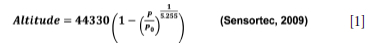
where P is the measured pressure, Po is the pressure at sea level, and the altitude is then given in metres. In this equation, a pressure change of 1 hPa equates to a change in altitude of approximately 8.4 m at sea level.

To confirm the accuracy and suitability of the sensor for obtaining usable data for incline and topographic profile, three simple indoor tests were performed.

Test 1: Barometric altitude vs. time (to investigate drifting of the altitude values over time)

For test 1 the sensor was left stationary on a table and the data was recorded over a period of 24 hours. The resulting plot can be seen in Figure 1, top left. It is noticed that the absolute altitude varied by as much as 60 m over a 24 hour period. This means that the absolute value for barometric altitude is not suitable for determining inclines of normal road profiles. When viewing the barometric pressure over a shorter time-frame (Figure 1, top right) one can see that the effect of the drift is much less (typically around 0.1 m per minute). From this result it was decided to use the relative altitude between two adjacent points rather than the absolute altitude value.

 

 

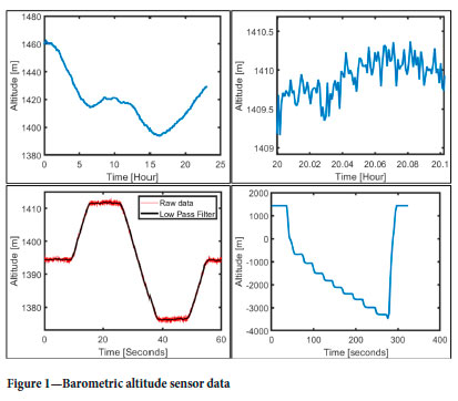
Test 2: Barometric altitude during an elevator ride (to verify the sensor's ability to smoothly detect small altitude changes)

The altitude was recorded when riding in an elevator from floor 9 up to floor 15, down to floor 3, and back to 9 again (Figure 1, bottom left). The red line is the raw data and the black line is a digital low-pass filter applied to the data afterwards. It is noted that the noise in short time-frames for the low-pass filtered data amounts to less than 0.75 m. For a 100 m stretch the noise equates to an incline angle error of less than 0.5°. This shows that the barometric data is sufficiently sensitive to determine an approximate topographic profile for a route, as the ranges typically experienced are significantly larger than the sensor's resolution on barometric altitude. It is, however, noted that this sensor's minimum detectable height does place a limitation on the shortest distance increment for which it can be used to effectively determine incline.

Test 3: Maximum simulated depth (to verify that the sensor can work in a deep underground mine)

The whole testing device was installed in a sealed container and incrementally pressurized up to a maximum absolute pressure of 1.5 bar. A pressure of 1.35 bar absolute equates to the pressure at the bottom of the deepest mine in the world at the time of this study, 2500 m below sea level, therefore slightly exceeding this deepest effective pressure would suffice to prove the device's ability to function as required (Mining Technology, 2019). The results for test 3 are shown in Figure 1, bottom right. It is seen that the sensor behaved in a predictable manner and gave the effective depth values as expected, returning back to the test location altitude again after the test, showing that no sensor damage occurred. This is a simple overpressure test to determine if the sensor can still yield sensible data at elevated pressures and is not intended as a detailed calibration test.

The barometric pressure sensor could now be implemented on a roadgoing vehicle that has an optical encoder to measure wheel displacement. This data can be used to obtain an estimation for the topographic plot for a route and to perform route identification. To have an above-ground comparison for the barometric altitude topographic plot and verify its usability, a GPS sensor was used to log the GPS coordinates (latitude, longitude, and altitude) as well. It was, however, noted that the barometric altitude shows jumps of tens of metres in the data when the sensor is exposed to direct sunlight, so special care should be taken to avoid these sudden changes in sensor temperature.

Heading data acquisition

Alvarez-Santos et al. (2015) obtained an estimate for heading from a three-axis magnetic sensor. A magnetic sensor is a low-cost sensor that can give the orientation of a device. The drawback is that it is easily affected by external magnetic field disturbances like electric motors and metallic objects. Gallant and Marshall (2016) propose a wheel rotation encoder to enable the heading data to be recorded as a function of distance.

The HMC5883L included on the GY-89 module board is a high-resolution three-axis magneto resistive sensor that can determine heading accurately within 1° to 2° using its built-in 12-bit analog-to-digital converter. The sensor has a maximum sampling rate of 160 Hz, which allows for multiple samples to be taken consecutively to average/filter out higher frequency noise in the sensor. The sensor can also be used in a strong magnetic field environment and still yield good heading accuracy as long as compensation is performed for the constant offsets (Honeywell International Inc., 2013). The heading noise of the raw data recorded by this sensor was found during testing to be approximately 0.5°.

Odometer

Initial testing was carried out using an instrumented road vehicle above ground and an instrumented handheld surveyor's wheel underground. These test platforms were both fitted with an optical encoder to obtain displacements over the routes in real time. As the odometer processor is fitted with a high-speed clock it is able to yield velocity as a function of distance and time, which is useful in calculations relating to the route energy, but that is outside the scope of this paper.

GPS as reference for odometer, velocity, and barometric altitude

To demonstate that the barometric pressure sensor is able to obtain an accurate topographic plot for a route and to be able to calibrate the odometer, the results must be verified using a good reference. As all of the initial tests of the RIS were performed above ground it was possible to use a GPS. The GPS module used is capable of obtaining a horizontal position accurately to less than 2.5 m and velocity with an error of less than 0.1 m/s. Boroujeni, Frey, and Sandhu (2013) found that GPS data is unreliable under bridges and overpasses, which was also found to be true during road tests in this study, especially when driving into a multi-level parking garage.

It was now possible to gather the topographic data for a route travelled by a road vehicle and compare the results to a GPS reference. The patterns in this data could be used in conjunction with patterns in heading data for various routes to implement the proposed RIS.

 

Calculations, modelling of the route identification system

Data acquisition system

A pair of open-source Arduino prototyping boards were used to read and scale the data streamed from the sensors and in turn stream these values to a laptop that processed these values as input to the RIS (Arduino, 2005). One Arduino board was used as the master to facilitate serial communication between the sensors and the laptop, and the other was set up as a slave to serve as the odometer. Once the preset distance increment for sampling of the heading and altitude is reached it transmits the total recorded distance to the main Arduino board. It was found that a distance increment of 100 m yields good overall results. Upon receiving the distance value from the odometer board the main Arduino board requests the heading and barometric altitude 20 times consecutively in a very short time-frame from each of the sensors to form a more stable averaged value for each parameter respectively. It then streams the averaged heading, averaged barometric altitude, and distance to the laptop via serial communication as a string. The 20 samples were found to yield stable enough data for use in subsequent processing. The sampling rates for these two sensors are high enough to allow multiple samples to be taken consecutively without a significant calculation time penalty or distance travelled over the sampling time. Figure 2 shows a schematic layout of the operation of the data acquisition system. Operating the stream in this way has the advantage that the amount of data that needs to be processed is low enough for the route identification program to be run in real-time.

 

 

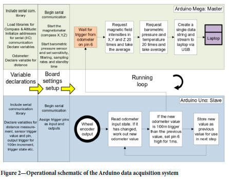
Figure 3a shows the GPS -altitude vs. -distance and the barometric altitude vs. optical encoder distance. It should be noted that the barometric altitude and the GPS altitude were zeroed at the start of the run to align with each other; the barometric drift was explained in the section on topography. The barometric data lines up very well with the GPS data. Figure 3b shows the zeroed barometric altitude vs. distance for the same route driven on three separate days, demonstrating very good consistency between the three tests.

 

 

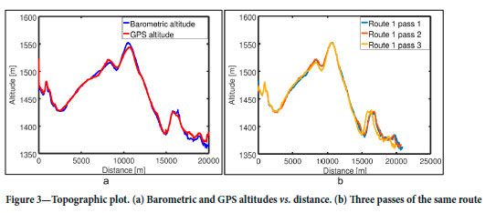
The GPS data signal is not without fault, as there is a large jump at the end of the data, and many times missing data was observed when travelling underneath a bridge/overpass. The jump at the end of the data was caused by the vehicle entering a covered parking building, thus degrading the GPS signal.

To alleviate the issue of zeroing the barometric altitude, which varies with weather conditions, and thus the absolute altitude accuracy, it makes sense to rather use the derivative of the function, i.e. the change in altitude over a predefined relatively short distance/ time increment. Altitude gain/loss over a small distance in a relatively short time will not noticeably suffer from weather and other environmental effects, as was shown in Figure 1. Figure 4a shows the raw incremental change in barometric altitude, which is termed the altitude gain, for three passes of the same route. The altitude gain also allows direct calculation of the incline of the route, which is beneficial for energy calculations performed in further studies.

 

 

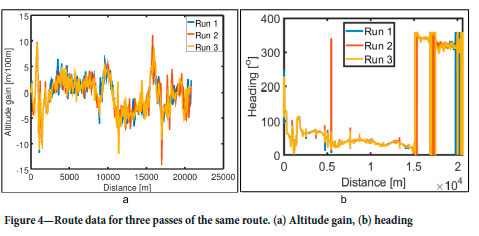
The heading was also recorded for the three passes to demonstate good correlation between the data for the same route on different passes; this is shown in Figure 4b. It is noted that the heading data shows very good consistency for the three passes. Headings near magnetic north are the cause for the abrupt jumps in the data from 15 000 m to the end. As an example a heading of 1° is only 2° away from a heading of 359°, and though it isn't intuitive from observing the figure it is easily accounted for in a later step when the comparisons between routes are done in the Results section.

Above-ground tests

The aim was to develop a system capable of identifying the route that is being travelled based on patterns in heading and altitude change data. Once these parameters had been recorded above ground and found successful in route identification the system could be tested for underground use. An distance increment of 100 m reduces the amount of data that requires processing compared to higher sampling rates and also reduces noise in the altitude gain data. The low sampling rate has one drawback; when the heading or altitude changes sharply, like on a residential winding road, it will degrade the ability to perform route identification as the exact location of the sample point around a bend is not the same from one pass of the route to the next, which will lead to significant differences in heading data.

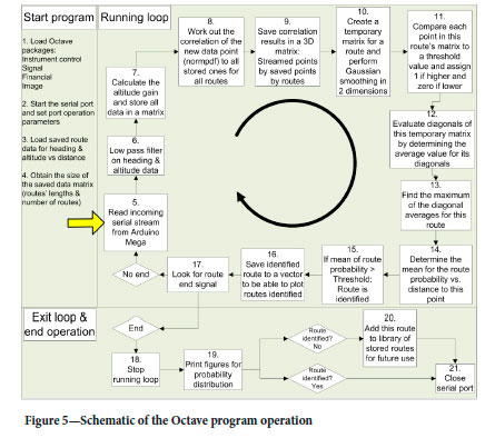
If the topographic plot of a certain route and the vehicle's location on that route are known, the hybrid vehicle control system is able to make better decisions regarding total energy management, a topic that is still under investigation by the authors. This study is based on an underground railway vehicle, so the route options are fairly limited compared to normal road vehicles which can do u-turns and take -side roads, thus greatly reducing the number of possible routes to search for. This limits the number of routes possible during route identification, and this will facilitate the development of an optimization system in future research. Figure 5 shows a schematic diagram of how the route identification program works. The program is excecuted in real time on a standard laptop. The software used is open-source GNU Octave v.4.2.1. (GNU Octave, 2017). These steps are explained in the paragraphs to follow.

 

 

A real-time route comparison can be performed only if there is information available for, at the very least, one route previously travelled. The first route was saved from the data recorded for the feasibility study of the heading and altitude change data. This data was saved in two text files, one containing the heading and the other the altitude gain information. With the distance increment being constant at 100 m it allows the heading and altitude data to be saved without their distance reference, as each new line of saved data is by design stored at the corresponding distance increment for comparison to the real-time data streaming in.

With each new heading and altitude data-point streamed in, the laptop in the vehicle is able to compare these new values to the recorded set of values for routes previously travelled and saved. The program makes use of a normal distribution function to yield a high value for good correlation and very low value for bad correlation. Each new data-point is compared to the data-points for all the previously saved routes on a point-by-point basis. Although this is a

tedious process, computationally speaking it is easily accomplished before the next data-points are streamed in a couple of seconds later. There is an advantage of always comparing all of the points of all of the routes as this allows the route identification program to identify a route even if the starting points do not line up, or to distinguish between routes that may have the same or very similar portions. Points are compared by calculating the value of the probability density function at point X of the normal distribution with a mean of μ and a standard deviation of σ. The variable X is the incoming data-point, μ is the saved data-point's value, and a is the standard deviation. The value for the standard deviation, a, was assumed to be constant, which was demonstrated to work well during simulations of the RIS. The OCTAVE/MATLAB function that is used for this is normpdf(X,μ,σ). This is not a purely statistical method; however, the normpdf function is a very convenient method of comparing the correlation between data-points. It is normalized for each data-point to ensure that the maximum probability density function value given by the function cannot exceed 1.0 for an exact match. A sensitivity analysis was performed to determine the best values for a based on route identification success rates. A low value for a will make the route identification program stricter, up to a point where no routes are ever identified as very few points will have exactly the same heading and altitude gain values, and a high value has the opposite effect where routes would be identified incorrectly. For the simulations performed a value of a = 8° was found to perform well for heading and a height change of a = 3 m per 100 m performed well for the altitude gain.

The altitude gain correlation value for a point streamed in is compared directly to all of the points in all of the saved routes. This will yield a N x M matrix which contains the correlation values, with N being in the direction of the data for the saved routes and M the data in the streamed-in route direction. The same point-for-point method is performed for the heading data, but additional computations need to be carried out. For the heading correlation it is necessary to specifically account for headings close to north, as was shown earlier (Figure 4b). This correlation matrix is generated by taking the probability for each heading point streamed in to the saved routes' values, and then doing the same again but this time using a heading value of (heading - 360°). This will allow a 358° incoming point to also be calculated as -2°. A third scenario is also applied where (heading + 360°) is used so that a streamed heading value of 1° can be compared to a saved value close to, but less than, 360°. The largest of these three heading correlation values for each point is stored in the heading correlation matrix and used in further calculation steps.

Now that a correlation value is determined for both the heading and altitude gain, point-for-point for all of the saved data-points, a resultant correlation matrix accounting for both heading and altitude gain at the same time is determined by simply multiplying the two correlation matrices, point-for-point. Thus, only if both the heading and the altitude gain data-points correspond well to the saved data-point does it register as a high correlation. These correlation values are recorded and saved in a 3D matrix, where one axis represents the number of routes evaluated, the second represents the streamed data, and the third axis the saved data.

If the route being travelled correlates to one of the saved routes, there will be a high band in the route's plane in the 3D matrix. The streamed data and saved data will have to be in phase with each other and yield consistently high correlation values for a route to be identified. The route planes in the 3D matrix are evaluated by taking the averages of bands in these matrices, where the bands are identified as Matrix(a+X,a). The value for 'a' ranges from unity up to the shortest length of the plane and 'X' is varied from the negative of half of the shortest length to the positive of half of that length. This in effect determines the averages for lines parallel to the diagonal of the matrix. The reason for not going all the way to the end of the matrix will be explained in more detail later.

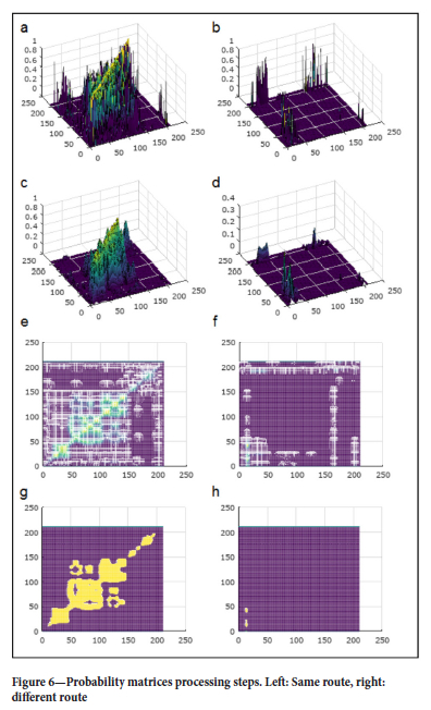
Figure 6a shows the resultant correlation matrix plotted for a case when the data of the route travelled is compared to itself. Figure 6b shows the travelled route compared to a different route stored. No pattern is apparent for the mismatched route, which is exactly what we expected. The bands are only evaluated in a positive direction in both the saved and streamed data axis as we are not evaluating travelling the route backwards at this stage. A band that has a consistently high correlation indicates a good chance of travelling on the specific saved route to which it is being compared. Not only the central band, but also bands parallel to that, need to be evaluated as the exact start points for the saved and streamed routes do not have to match. tt is importand to evaluate the parallel bands as this will allow route identification even when the starting points of the routes are not the same, or when there are slight distance discrepancies between the saved and current test streams. There is, however, a limit to the minimum distance that a route needs to correlate with before it is claimed as identified. This restriction is necessary to neglect the false positive route identifications that arise if only a couple of consecutive points line up close to the start or end. If the program was not able to establish a good correlation between the travelled route and any of the saved routes, it was set up to then save this route as a new route, the data for which will be used in the route identification steps in future passes.

 

 

It is of benefit if the RIS is somewhat lenient in terms of the exact band that correlates to a route. For example, if a set of data is offset by 50 m relative to the saved route it might cause the high band values to float between two adjacent bands, depending on the exact point being considered, which will cause the band's average value to drop drastically, even though the same route is being travelled. This situation can occur due to wheel slippage, or slight offsets in the starting points. The strategy implemented to make route identification more forgiving and robust is to make use of a smoothing filter on the route's correlation matrix, which means that a route can be identified even if there does not exist a single band with high correlation values. A Gaussian filter was implemented for this purpose. This filter will also pull up local low points that might have been caused by a local error, for example when travelling around a sharp corner and the two data-points which are being compared don't line up perfectly around the corner, yielding almost zero correlation for that local point due to the heading correlation value being far off.

The smoothed data is shown in Figures 6c and 6d, for the same and another route respectively. This smoothing strategy reduces the effect of starting value differences, small amounts of wheel slip, and other factors that cause the exact distance correlations to deviate from the single high band. A point to note, however, is that this smoothing filter also reduces the maximum probability value for a route point which correspond 100%, due to the neighbouring ones that draw it down slightly. Figures 6e and 6f shows plan views of the smoothed probabilities for the same route (e) and another route (f). A high correlation band is clear for the similar route (e) and no high bands are visible for the other route (f). A potential issue with evaluating the bands based only on the highest average value could be that a band with a consistent medium probability might be outweighed by a diagonal with generally low probability and some local high probabilities, or some consistently low route may even end up being the highest average probability and incorrectly identified as a route, simply because it happened to be the highest probability of the data available. To avoid this potential error in averaging of correlation values a threshold value to the probabilistic matrix was applied, causing the probability for a point to simply be considered as either zero (no correlation) or unity (sufficient match), based on some experimentally determined constant threshold cut-off value. This process is illustrated in Figures 6g and 6h. Now the band values can be compared and if found to exceed a preset value it can be assumed a positively identified route.

To avoid erroneous route identifications based on the average band approach it is important to stay in the central region of the matrix, and not to calculate the averages for the extreme end points. For example, if a distance travelled equal to the final point of the route is considered, in the real-time program no further information regarding the route will be available yet, and thus the diagonal average value for the end point of the matrix, with a length of one cell, might have an average = 1, which is the maximum value and thus the route will be 'confidently' identified based on a single data-point. This will lead to many incorrect route identifications and make the whole system unstable. To alleviate this problem not all of the bands are considered, but only those in the central region. For the purpose of the tests it was found that using half of the matrix width in either direction for the bands mostly solved this problem of incorrect/erratic route identification. In general, route identification more than halfway through the route would not be very beneficial in an optimization strategy in any way. If, by the end of a route no routes were identified the system automatically saves this route as a new route that will be used in future passes to perform route identification.

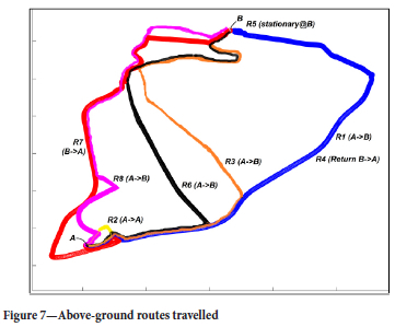
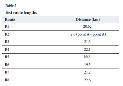
Eight routes were used to evaluate the effectiveness of the RIS. Most of the routes were back and forth between points A and B (Figure 7). These routes were plotted from the GPS data recorded during testing. It should be noted that the routes overlap close to the start and end points, so initial identification of a route may be incorrect as it is impossible to tell where you are going to turn off and continue with the planned route. It is important to remember this when the route optimization is performed later on as it directly influences the route optimization that needs to be performed and can be detrimental to optimizing if the incorrect route is optimized for initially. Most of these routes are tarmac public roads. Route R5 is a table-top test, where the distance travelled is theoretically simulated, although no real movement took place. The advantage of using the constant valued route R5 is that it facilitated fault-finding and refinement of the program during tests/simulations performed without physical testing on the road. The trip distances of the routes between A to B are stated in Table I. Route 2 was an around-the-block route to verify sensor data and was not travelled for route identification purposes.

 

 

 

 

A sensitivity analysis was performed through simulations and the most usable and safe values for accurate route identification are as follows: σ_{Altitude gain} = 3 m per 100 m, σ_Heading = 8°, and threshold cut-off value = 0.2. These values were then used to perform above-ground real-time route identification for the eight routes. The results are presented in the Results and discussion section.

Underground tests

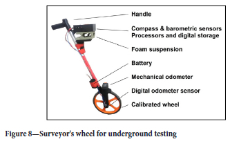
Gathering of vehicular test data in an operating underground mine was not possible due to security and safety concerns. The best alternative was to build a small handheld device that could be used to record heading vs. distance and altitude vs. distance data in an underground environment to prove that these parameters can be effectively measured underground and form patterns that yield the same RIS success as was obtained above ground. The handheld device used for the underground tests was an instrumented surveyor's wheel fitted with an optical encoder, magnetometer, and barometric pressure sensor, but in this case the real-time data was recorded on a SD card and processing afterwards due to space and practical reasons. Figure 8 shows the handheld device. At the bottom of the device, just above the wheel, is the battery. The battery needed to be placed far away from the magnetometer as it was found that close proximity causes a catastrophic offset in the heading data, rendering the whole test unusable unless the magnetometer was specifically recalibrated for this offset. The magnetometer/barometer were mounted on top of a skeletonized soft foam suspension block to reduce accelerations on the sensor, which were found to increase data noise in the barometric pressure sensor. The surveyor's wheel has a factory-calibrated distance readout, which made calibration and quality checking of the recorded data much easier. For the above-ground tests the distance increment was set to 100 m, but in the tests with the handheld device the distance increment was reduced to 5 m, as walking many kilometers underground is not very practical. It was recognized that the altitude data will now yield noisy incline data due to the minimum elevation accuracy mentioned in the topography section.

 

 

It had already been proven that the heading and altitude gain strategy works above ground, so in-detail underground tests were not deemed essential, rather, simply to prove the device's ability to detect appropriate heading and barometric values underground so that route identification can be performed.

Basement parking lot test

The first underground tests were performed in the basement parking of the Engineering 3 building, at the University of Pretoria's main campus, on level P1, two levels below ground level. The building is a steel-reinforced concrete structure with no external steel structural members. Mentioning this is important as it could have an effect on the magnetic data. A circuit on level 1 was walked four times with the device reset at approximately the same point on each pass. The circuit started on a flat section, proceded down a slope, back up the slope again and on the flat to the start point of the route. The results for route identification in the basement tests are included in the Results and discussion section.

Gold mine underground testing

The testing of the device to determine if it functions in an actual gold mine was performed at Gold Reef City, an amusement park located in Johannesburg, South Africa. There is a decommissioned small gold mine on site, which is now only used for tourist and educational visits. The purpose of performing a test in a real mine, though it is very small compared to the commercially active mines, was to verify that the sensors yield information that can be used to successfully perform route identification. The same surveyor's wheel set-up that was used for the basement test was used for the underground mine test. The mine's tourist level is located approximately 76 m below the surface. Only two passes were granted for testing purposes. The results for the route identification performed in the Gold Reef City mine are presented in the next section.

 

Results and discussion

Above-ground route identification

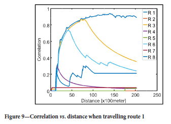
Eight different routes were evaluated. Route 2 was just a short test route to evaluate sensor function and the data being streamed. Route 5 was a theoretically generated constant route to allow finer testing of the system. In Figure 9 the route correlation values are plotted against distance for all of the saved routes when travelling on route 1. It is noted from Figure 7 that routes 1, 3, and 6 all have the same initial portions, which is why it makes sense that routes 3 and 6 both also had increasing correlations up to the point where they deviate from route 1. This proves that the RIS was able to correctly identify the route travelled with high confidence by 4.6 km, equating to less than 20% of the total route length, and with moderate confidence by 2.5km.

 

 

Route identification tests were performed multiple times for every real route to evaluate the ability of the RIS to perform satisfactorily. Table II summarizes the results, showing the route travelled, the route identified, along with the distance where it was identified and the number of times each route was tested.

 

 

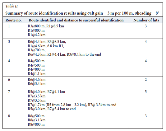
From the test results shown in Table II it is seen that the RIS was able to identify the correct route in every test performed, in real time, with small errors occationally found in the initial parts of the routes. In the case of route 7, route 5 was twice identified initially for short parts of the route due to similarities between the routes' data, though this error was corrected within 400 m and the correct route was maintained until the end.

The reason why the identification correlation value starts at zero is due to the program being set up such that it starts at zero for all routes so as not to favour any route above another without proper knowledge of the route being travelled. With it using an averaging program the initial zero correlation gradually grows as the correlation of the route with a stored one increases over distance. The routes are usually more winding at the start and towards the destination due to parking lot driving and sharp corners followed in residential areas, where the under-sampling of the route data at 100 mr increments reduces the ability of the RIS to lock onto a route.

The ability of this system to run in real -time allows the RIS to not only identify the route being travelled but also to know the location of the vehicle on that route (route progress), which will be essential when optimizing the energy management of a hybrid locomotive in further studies.

Basement test results

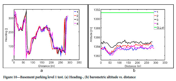
The heading and altitude data for these passes can be seen in Figures 10a and 10b respectively. Good consistency is seen in the data for the four passes. It should be noted that, being obtaines by hand, this data will not be as consistent as that obtained by a vehicle driving on a public road with lane directions clearly indicated and closely adhered to, and even less than what a rail-bound locomotive will see.

 

 

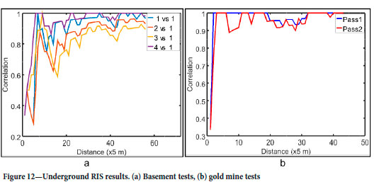
Four passes of the same route were used for the test. The first one was saved as the reference, with all four routes compared to this stored route. Comparing the route to itself is handy for consistency checking. Figure 12a shows the correlation as a function of the distance (5 m increment). It is seen that the route that was walked four times yields data that is usable for the RIS proposed. The noise introduced due to manual operation did reduce the smoothness of the correlation graphs, as is expected. The reason why a 100% probability is not achieved with route 1 compared to itself is due to the Gaussian filter, as was explained in the above-ground tests section.

 

 

 

 

It could now be concluded that the RIS yields satisfactory results for an underground basement test using the handheld data logging device. The next step was to perform tests in a mine, located at greater depths and in the typical rocks that mines are excavated in to confirm applicability of this system in underground environments.

Gold Reef City underground test results

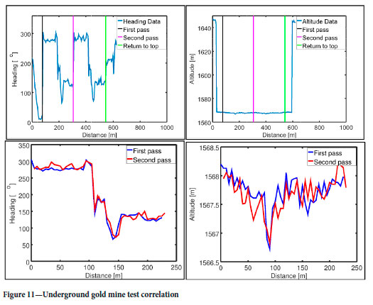
Only two passes were granted in a small underground gold mine on the tourist level to determine whether the heading and altitude data can be used to identify a route being travelled. In the top of Figure 11 the sensor data can be seen for a trip from the surface, twice through the mine's underground visitor's loop, and back to the surface. It is noted that the initial change in heading was as we approached the elevator shaft, and the jump on the vertical black line is due to us walking out of the elevator in the opposite direction with the test data for the first pass starting directly after that. There is also a jump in the altitude data as the elevator descended . The data is then split into the two individual passes plotted over each other. The progress stages are indicated by the three vertical lines in the top of figure. The altitude is shown in this case instead of the altitude gain as the noise is too great on the small distance increments used, making it difficulte to see any patterns.

In the bottom left of Figure 11 it can be seen that the heading data is very closely correlated between the two passes. The altitude data shows good correlation as well, although the data is much more noisy when one zooms into the local values. The noise in the data amounted to around 0.5 m, which corresponds to the accuracy stated previously. The route identification algorithm can be set up to allow for higher noise in the barometric data by using less strict statistical parameters (larger σ value). Though it is noisy this does still enable comparison of patterns in the data.

The correlation vs. distance plots for the underground gold mine tests are given in Figure 12b. Pass 1 is compared to itself and then to the second pass. The correlation is not 100% all the way through due to the Gaussian filter, as discussed previously. It can be seen that the RIS very quickly identifies pass 2 as the same route as pass 1, taking only around four samples, which equates to a distance of 20 m, or less than 10% of the loop distance, and consistently identifyes the route from there onwards with high confidence.

 

Conclusion, recomendations, and future work

A novel method of identifying routes underground and finding the location on a route has been presented. This method makes use of easily and affordably obtained magnetic heading and barometric altitude values measured as a function of distance while driving the route. This automatically also yields a topographic profile for the route, which can be used in later processing for route optimization. A pattern recognition program was developed that is able to compare patterns in data for a route being driven to a set of routes that were driven previously and which is stored into a simple small text file in memory. This strategy was able to successfully identify a route being travelled by a vehicle, as well as the location of the vehicle on that route, for a total of six real-life route options investigated. The location on the route is known simply by the most recent data-point streamed in, once the route is identified If the route is not known to the system it is automatically saved as a new route to the small text file, which will then be used for route identification comparisons in future driving cycles. The system proved to function both above ground and underground, where GPS signals are not available. A sensitivity analysis was able to identify the optimal parameters for which the route identification strategy yielded the best results. The route identification strategy was able to always converge to the correct route within a short distance, typically within the first 20% of the route travelled.

For future work the standard deviation value for each point of the route can be updated based on the stability of the streamed data for that that portion of the route, and through averaging the data for many passes of the same section. This has the potential to improve the route identification accuracy and responsiveness. If the system is implemented in an actual deep underground mine the absolute pressure obtained by the barometric pressure sensor can also be used to rule out certain routes from the stored set for that mine, as mine levels are usually many metres apart, which will lead to reduced calculation times. When using a route identification strategy to optimize route energy management it is crucial to take into account the fact that the initial parts of some routes are similar and thus optimizing for a specific route can be detremental to the efficient completion of another which the vehicle could potentially be travelling at that time, and one can only fully optimize when enough certainty on route uniqueness is obtained.

 

Acknowledgements

The author would like to thank Gold Reef City theme park for their kind assistance in allowing undergound testing at their facility.

 

References

Alvarez-Santos, V., Canedo-Rodriguez, A., Iglesias, R., Pardo, X.M., and Regueiro, C.V. 2015. Route learning and reproduction in a tour-guide robot. Robotics and Autonomous Systems, vol. 63. pp. 206-213. https://doi.org/10.1016/j.robot.2014.07.013        [ Links ]

Arduino, I.I.D.I. 2005. Arduino IDE. GitHub. https://www.arduin.cc/en/software        [ Links ]

Back, M., Simons, M., Kirshaum, F., and Krebs, V. 2002. Predictive control of drivetrains. IFAC Proceedings Volumes, vol. 35, no. 1. pp. 241-246. https://doi.org/10.3182/20020721-6-ES-1901.01508        [ Links ]

Basso, R., Kulczár, B., Ehardt, B., Lindroth, P., and Sanchez-Diaz, I. 2019. Energy consumption estimation integrated into the Electric Vehicle Routing Problem. Transportation Research Part D: Transport and Environment, vol. 69. pp. 141-167. https://doi.org/10.1016/j.trd.2019.01.006        [ Links ]

Bender, F.A., Kaszynski, M., and Sawodny, O. 2013. Drive cycle prediction and energy management optimization for hybrid hydraulic vehicles. IEEE Transactions on Vehicular Technology, vol. 62, no. 8. pp. 3581-3592. https://doi.org/10.1109/TVT.2013.2259645        [ Links ]

Boriboonsomsin, K. and Barth, M. 2009. Impacts of road grade on fuel consumption and carbon dioxide emissions evidenced by use of advanced navigation systems. Transportation Research Record: Journal of the Transportation Research Board, vol. 2139, no. 1. pp. 21-30. https://doi.org/10.3141/2139-03        [ Links ]

Boroujeni, B.Y., Frey, H.C., and Sandhu, G.S. 2013. Road grade measurement using in-vehicle, stand-alone GPS with barometric altimeter. Journal of Transportation Engineering, vol. 139, no. 6. pp. 605-611. https://doi.org/10.1061/(ASCE)TE.1943-5436.0000545        [ Links ]

Boyd, S. and Nelson, D.J. 2008. Hybrid electric vehicle control strategy based on power loss calculations. Proceedings of the SAE World Congress & Exhibition. https://doi.org/10.4271/2008-01-0084        [ Links ]

Chen, Z., Li, L., Yan, B., Yang, C., Ma, C.M., and Cao, D. 2016. Multimode energy management for plug-in hybrid electric buses based on driving cycles prediction. IEEE Transactions on Intelligent Transportation Systems, vol . 17, no. 10., pp. 2811-2821. https://doi.org/10.1109/TITS.2016.2527244        [ Links ]

CMTi Group. 2021. LOCO1000 Series. http://cmtigroup.co.za/LOCO1000-Series/ [accessed 7 September 2021.         [ Links ]

Gallant, M.J. and Marshall, J. A. 2016. The LiDAR compass: Extremely lightweight heading estimation with axis maps. Robotics and Autonomous Systems, vol. 82. pp. 35-45. https://doi.org/10.1016/j.robot.2016.04.005        [ Links ]

GNU Octave. 2017. GNU Octave. https://www.gnu.org/software/octave/ [accessed: 19 November 2019].         [ Links ]

Hellström, E., Âslund, J., and Nielsen, L. 2010. Design of an efficient algorithm for fuel-optimal look-ahead control. Control Engineering Practice, vol. 18, no. 11. pp. 1318-1327. https://doi.org/10.1016/j.conengprac.2009.12.008        [ Links ]

Honeywell International Inc. 2013. HMC5883L_3-Axis_Digital_Compass_IC.pdf        [ Links ]

Hu, X., Martinez, C.M., and Yang, Y. 2017. Charging, power management, and battery degradation mitigation in plug-in hybrid electric vehicles: A unified cost-optimal approach. Mechanical Systems and Signal Processing, vol. 87. pp. 4-16. https://doi.org/10.1016/j.ymssp.2016.03.004        [ Links ]

Huang, Y., Wang, H., Khajepour, A., He, H., and Ji, J. 2017. Model predictive control power management strategies for HEVs: A review. Journal of Power Sources, vol. 341. pp. 91-106. https://doi.org/10.1016/j.jpowsour.2016.11.106        [ Links ]

Jeon, S., Jo, S., Park, Y., and Lee, J. 2002. Multi-mode driving control of a parallel hybrid electric vehicle using driving pattern recognition. Journal of Dynamic Systems, Measurement, and Control, vol. 124, no. 1. p. 141. https://doi.org/10.1115/1.1434264        [ Links ]

Johannesson, L., Murgovski, N., Jonasson, E., Hellgren, J., and Egardt, B. 2015. Predictive energy management of hybrid long-haul trucks. Control Engineering Practice, vol. 41. pp. 83-97. https://doi.org/10.1016/j.conengprac.2015.04.014        [ Links ]

Lajunen, A. 2014. Fuel economy analysis of conventional and hybrid heavy vehicle combinations over real-world operating routes. Transportation Research Part D: Transport and Environment, vol. 31. pp. 70-84. https://doi.org/10.1016/j.trd.2014.05.023        [ Links ]

Lin, C.-C., Jeon, S., Pemg, H., and Lee, J.M. 2004. Driving pattern recognition for control of hybrid electric trucks. Vehicle System Dynamics, vol. 42, no. 1-2. pp. 41-58. https://doi.org/10.1080/00423110412331291553        [ Links ]

Liu, H., Li, H., Rodgers, M.O., and Guensler, R. 2018. Development of road grade data using the United States geological survey digital elevation model. Transportation Research Part C: Emerging Technologies, vol. 92. pp. 243-257. https://doi.org/10.1016/j.trc.2018.05.004        [ Links ]

Mining Technology. 2019. Top ten deepest mines in the world. https://www.mining-technology.com/features/feature-top-ten-deepest-mines-world-south-africa/ [accessed: 19 November 2019].         [ Links ]

Phillips, A.M., Jankovic, M., and Bailey, K.E. 2000. 'Vehicle system controller design for a hybrid electric vehicle. Proceedings of the 2000. IEEE International Conference on Control Applications. Conference Proceedings (Cat. No.00CH37162). 2000 IEEE International Conference on Control Applications, Anchorage, AK: IEEE. pp. 297-302. https://doi.org/10.1109/CCA.2000.897440        [ Links ]

Rezaei, S. and Sengupta, R. 2007. Kalman filter-based integration of DGPS and vehicle sensors for localization. IEEE Transactions on Control Systems Technology, vol. 15, no. 6. pp. 1080-1088. https://doi.org/10.1109/TCST.2006.886439        [ Links ]

Rogers, K.J. and Trayford, R.S. 1984. Grade measurement with an instrumented car. Transportation Research Part B: Methodological, vol. 18, no. 3. pp. 247-254. https://doi.org/10.1016/0191-2615(84)90035-3        [ Links ]

Sensortec. 2009. BMP085 Digital pressure sensor. p. 27.         [ Links ]

Song, K., Li, F., Hu, X., He, L., Niu, W., Lu, S., and Zhang, T. 2018. Multi-mode energy management strategy for fuel cell electric vehicles based on driving pattern identification using learning vector quantization neural network algorithm. Journal of Power Sources, vol. 389. pp. 230-239. https://doi.org/10.1016/j.jpowsour.2018.04.024        [ Links ]

Taghavipour, A., Vajedi, M., Azad, N.L., and McPhee, J. 2016. A comparative analysis of route-based energy management systems for Phevs: Asian Journal of Control, vol. 18, no. 1. pp. 29-39. https://doi.org/10.1002/asjc.1191        [ Links ]

Tie, S.F. and Tan, C.W. 2013. A review of energy sources and energy management system in electric vehicles. Renewable and Sustainable Energy Reviews, vol. 20. pp. 82-102. https://doi.org/10.1016/j.rser.2012.11.077        [ Links ]

Vahidi, A., Stefanopoulou, A., and Peng, H. 2005. Recursive least squares with forgetting for online estimation of vehicle mass and road grade: theory and experiments. Vehicle System Dynamics, vol. 43, no. 1. pp. 31-55. https://doi.org/10.1080/00423110412331290446        [ Links ]

Wang, R. and Lukic, S.M. 2011. Review of driving conditions prediction and driving style recognition based control algorithms for hybrid electric vehicles. Proceedings of the IEEE Vehicle Power and Propulsion Conference, Chicago, IL, USA. pp. 1-7. https://doi.org/10.1109/VPPC.2011.6043061        [ Links ]

Yokoi, Y., Ichikawa, S., Doki, S., Okuma, S., Naitou, T., Shilmado, T., and Miki, N. 2004. Driving pattern prediction for an energy management system of hybrid electric vehicles in a specific driving course. Proceedings of the 30th Annual Conference of IEEE Industrial Electronics Society, IECON 2004, Busan, South Korea: IEEE. pp. 1727-1732. https://doi.org/10.1109/IECON.2004.1431842        [ Links ]

 

 

Correspondence:
R.F. Meeser
Email: riaan.meeser@up.ac.za

Received: 4 Nov. 2021
Revised: 21 Oct. 2022
Accepted: 15 Nov. 2022
Published: January 2023