PROFESSIONAL TECHNNICAL AND SCIENTIFIC PAPERS

 

A simulation model to study truck-allocation options

 

 

W. Zeng^I; E.Y. Baafi^I; H. Fan^II

^ISchool of Civil, Mining and Environmental Engineering, University of Wollongong, Australia. ORCID: W. Zeng: https://orcid.org/0000-0003-4689-003X
^IIJilin University of Finance and Economics, China

Correspondence

 

 

---

SYNOPSIS

We present a discrete event simulator, TSJSim (Truck-Shovel JaamSim Simulator), for evaluating the stochastic and dynamic operational variables in a truck-shovel system. TSJSim offers four truck allocation strategies: Fixed truck assignment (FTA), Minimizing shovel production requirement (MSPR), Minimizing truck waiting time (MTWT), and Minimizing truck semi-cycle time (MTSCT) including the genetic algorithm (GA) optimization and the frozen dispatching algorithm (FDA) optimization rules. Multiple decision points along the haul routes for all the trucks close to the decision points were included in the model. The simulation results indicate that the trends associated with production tons and queuing time utilizing the four truck allocation strategies (MSPR, MTWT, FDA, and GA) all demonstrated similar patterns as the fleet size varied. As the system fleet size increased, the system production tons under these strategies at first increased significantly and then remained relatively constant; the queuing time relating to these strategies showed a positive relationship with the system fleet size. The bunching time decreased when the truck allocation strategies were applied in the model. In the simulated truck-shovel network system with multiple traffic intersections, by assigning the trucks at the intersections, both productivity and fleet utilization increased.

Keywords: truck-shovel system, simulation.,truck allocation strategy, optimization.

---

 

 

Introduction

For a truck-shovel system in an open pit mine, the truck haulage costs have been reported to exceed half of the total direct operating costs (Lizotte and Bonates, 1987). Truck allocation strategies have been applied to improve productivity and/or reduce operating cost by considering alternative truck-shovel assignments in real time in order to increase utilization of system resources (Alarie and Gamache, 2002). By allocating the optimal number of trucks to shovels, the waiting times of trucks in an over-trucked system as well as the idle times for shovels in an under-trucked system can be minimized (Baafi and Ataeepour, 1998). Furthermore, by re-routing trucks when traffic congestion occurs, costs associated with various delays can be minimized (Jaoua, Gamache, and Riopel, 2012b).

According to Alarie and Gamache (2002), the main forms of truck allocation are single stage and multistage systems. The single stage approach assigns trucks to shovels based on one or several criteria without considering any specific production targets or constraints. These criteria are usually heuristic methods based on rules of thumb (Alarie and Gamache, 2002), including fixed truck assignment (Lizotte and Bonates, 1987), minimizing truck waiting time (Baafi and Ataeepour, 1998), minimizing shovel idle time, maximizing truck momentary productivity, and minimizing shovel saturation (Kolonja, Kalasky, and Mutmansky, 1993). The multistage approach, on the other hand, consists of several stages or sub-problems (Afrapoli and Askari-Nasab, 2017), which can be usually reduced to an upper stage (i.e., a production optimization problem) and a lower stage (i.e., a real-time dispatching problem). The upper stage aims to set production targets for every shovel according to specific operational constraints, while the lower stage assigns trucks to shovels to minimize the deviation from the production targets set by the upper stage.

The approaches used to solve the production optimization problem in the truck-shovel dispatching models include linear programming (LP) (White and Olson, 1986; Lizotte and Bonates, 1987; Li, 1990; Gurgur, Dagdelen, and Artittong, 2011; Ta, Ingolfsson, and Doucette, 2013; Mena et al., 2013), nonlinear programming (NLP) (Soumis, Ethier, and Elbrond, 1990), goal programming (GP) (Temeng, 1997), and stochastic programming (Ta et al., 2005).

For the real-time dispatching problem, the model developed by White and Olson (1986) assigns trucks to shovels to minimize the deviation between the current path flow rate and the optimal path flow rate specified by the LP model. They created two assignment lists: the first for the trucks and the second for the paths. The dispatching is achieved by matching the 'best truck' from the truck list with the 'neediest path' from the path list considering the truck capacity, shovel digging rate, expected truck waiting time and travel time, and expected shovel idle time, etc. Elbrond and Soumis (1987) proposed a dispatching procedure that minimizes the sum of squared differences between the average waiting time of trucks and shovels as calculated from the haulage allocation plan and the forecast waiting times based on the current status of the mine operation. However, they did not consider the possibility of assigning more than one truck to a shovel in one decision-making step, and they also assumed that the truck fleet is homogeneous. Bonates and Lizotte (1988) proposed a dispatching method which takes the results from their developed simulator and compares these with an optimal production plan obtained from their LP model. The dispatching criterion with the smallest deviation of results from the optimum production target is chosen as the optimum dispatching rule. Li (1990) proposed a truck dispatching algorithm based on the difference between the actual truck interval time and the optimal truck interval time on a path to a destination. However, a significant disadvantage of this real-time dispatching model is that the truck waiting times at the destinations, especially at the shovels, are ignored. Temeng (1997) proposed a real-time dispatching model based on the transportation problem. In this model, needy shovels are defined as those shovels with current cumulative productions below the target obtained from their GP model. The number of trucks required by each needy shovel is determined by comparing the tonnage for each route required to maintain ore quality and stripping ratios with appropriate truck capacity. However, the model is not able to account for the truck waiting time, which depends on the previously allocated trucks, especially in an over-trucked system.

Ouelhadj and Petrovic (2009) suggested that the intelligent metaheuristic searching methods, including the genetic algorithm, Tabu search (Wu and Garcia de Soto, 2020), and simulated annealing, are more powerful and appropriate for complex system scheduling/control optimization than the simple heuristic rules. Pfeiffer, Kadar, and Monostori (2007) also demonstrated the performance improvement using a dynamic scheduling method based on a genetic algorithm. Jaoua, Gamache, and Riopel (2012a) proposed a metaheuristic model, using the simulated annealing (SA) algorithm to compute the near-optimal assignment in a truck-shovel dispatching system.

Discrete event simulation techniques have been widely used in the mining industry to "evaluate and analyse mining operations (Dindarloo, Osanloo, and Frimpong, 2015; Afrapoli and Askari-Nasab, 2017; Yilmaz and Erkayaoglu, 2021. Askari-Nasab, Frimpong, and Szymanski (2007) developed an open pit production simulator to represent dynamic expansion of an open pit mine. Fioroni et al. (2008) developed a discrete event simulator that works with an optimization model to implement the short-term production plan. Ebrahim et al. (2015) used GPSS/ H® to develop a discrete event system simulation for a truck-shovel system to investigate the environmental impact, taking into account mining haulage performance and production targets. Hashemi and Sattarvand (2015) developed a discrete event simulation model using Arena simulation software to evaluate the transportation system of a copper mine. Their model is able to monitor the material excavated from different operating benches and considers the -ore grade requirement. Upadhyay and Askari-Nasab (2017) developed a simulation optimization tool that interacts with a GP-based optimization model to generate an uncertainty-based short-term plan.

As identified by Afrapoli and Askari-Nasab (2017), there are still many shortfalls in the existing real-time dispatching algorithms and models. Two major limitations are how to model close to reality and how to determine dynamic best path. For large open-pit mines, there is a large fleet of heterogeneous trucks hauling on a vast network of haul roads in the operation area. Most previous work on simulation of a truck-shovel system (Lizotte and Bonates, 1987; Kolonja, Kalasky, and Mutmansky, 1993; Temeng, 1997; Baafi and Ataeepour, 1998; Hashemi and Sattarvand, 2015; Sofranko, Wittenberger, and Skvarekova, 2015; Que, Anani, and Awuah-Offei, 2016) failed to capture the interaction between the individual vehicles as well as the influence of the dynamic traffic network environment on the real-time truck allocation.

In this paper we present a discrete event simulation model, TSJSim (Truck-Shovel JaamSim Simulator) with the capabilities of evaluating the key performance indicators (KPIs) of a truck-shovel system under the influence of truck allocation strategies. TSJSim considers not only the stochastic and dynamic operational elements of the network system, but also the interaction between the individual trucks in the traffic network environment.

 

Main components of TSJSim

TSJSim was developed using an open source simulation software package, JaamSim (JaamSim, 2018). JaamSim provides the capability of developing new objects in the standard Java programming language. New objects can be programmed with 3D graphics along with the Input Editor and Output Viewer, and can be dragged-and-dropped for direct usage. Twelve new objects were developed for modelling a typical truck-shovel mining network system. The main simulation model objects are OreGenerator, OreSink, OreEntity, Truck, Loader, Dump, Queue, Route, Routelntersection, RouteSafeZone, Truck-allocationStrategy, and LoaderOperator. Further details about these model objects are provided in Zeng et al. (2016).,

In TSJSim, the dynamic interactions between the haul trucks (i.e., bunching) and between the trucks and the traffic environment (i.e., traffic intersection area and main route priority management) are implemented by the truck velocity module, the truck bunching module, and the intersection management module. Further details about these modules are provided in Zeng, Baafi,and Walker (2019 ).

 

TSJSim truck allocation approach

In this paper, a truck-allocation decision point is defined as the time or the spatial position at which a truck driver needs to make a decision as to what route to select so as get to a particular destination. This decision may occur before and after loading, before and after dumping, or when a truck arrives at an intersection.

Most of the previous simulation models assume one or two decision points in one truck cycle, either at the loading site or at the dump site or at both. For example, in DISPATCH (White and Olson, 1993), the trucks in the real-time dispatching list are those that have completed or are about to complete dumping; Hauck (1973) assumed the unloading point to be the decision point for real-time truck dispatching; Jaoua, Gamache, and Riopel (2012a) used a specified regular time interval (the control horizon) to manage the time for dispatching instead of using a decision point.

In the TSJSim simulation model, multiple decision points in the haulage network system within a one truck cycle were considered to handle the complexity of the traffic network and the dynamic operational variables of a surface mine. The Routelntersection object handles the assignment of the Truck on Route objects. Referring to a typical truck-shovel network system shown in Figure 1, an assignment is generated by the Truck-allocation Strategy object to send the Truck to a loading site. This scenario applies as a loaded Truck completes dumping at Dump 2. Moreover, this depends on the system status, e.g., the traffic conditions on the various Routes, the availabilities of the Shovels, the lengths of the Queues at the loading sites and the performance of the LoaderOperators.

 

 

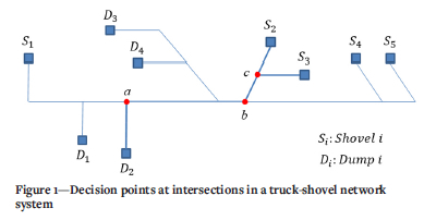
After hauling for a period of time, the Truck arrives at Routelntersection a, which provides an opportunity for the Truck to make a decision either to turn left for Shovel 1 or to turn right towards other Shovels {S_i, i = 2,3,4,5}. The system status when the Truck arrives at RouteIntersection a may be different from when the Truck was leaving Dump 2. If the Truck-allocation Strategy object regenerates a new truck-allocation solution at that moment, the assignment for the Truck may be different but could be more productive than the assignment when the Truck was leaving Dump 2. After hauling from Routelntersection a to b, the Truck then makes a further choice between Shovel 2, 3, 4 or 5. A similar decision is made when the Truck arrives at Routelntersection c, which is the last intersection on the haul route. Thus, it is clear that in a truckshovel network system where the operational variables change continuously, the truck assignment decisions could be made at the decision points on the haulage network to optimize productivity.

In the TSJSim simulation model, the truck-allocation approach is implemented mainly by two objects: the Routelntersection object and the Truck-allocation Strategy object. The Routelntersection object specifies all the decision points on Routes as well as the associated possible truck-allocation paths at each decision point. The Truck-allocation Strategy object assigns a Truck object to a destination based on the specified truck-allocation strategy.

Truck allocation paths development

The total possible truck-allocation paths for the trucks to travel from the traffic intersections to all the loading sites or dump sites are specified and stored in a list referred to as the RoutePool list in the Routelntersection object. For instance, Figure 2 shows an ideal truck-shovel haulage network layout with the decision points for the loaded trucks and the possible paths at the Routelntersection objects.

 

 

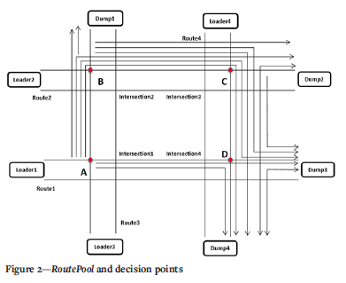
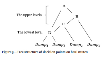
The RoutePool list at decision point D has two possible truck-allocation paths, i.e., D - Dump 3 and D - Dump 4; the RoutePool list at decision point C contains three possible paths, i.e., C -Dump 2, C -D - Dump 3, and C -D - Dump 4; the RoutePool list at decision point B includes four possible paths, i.e., B - Dump 1, B - C - Dump 2, B - C - D - Dump 3, and B - C - D - Dump 4; the RoutePool list at decision point A has six possible paths, i.e., A - B - Dump 1, A - B - C - Dump 2, A - B - C - D - Dump 3, A - B -C -D - Dump 4, A -D - Dump 3, and A -D - Dump 4. To determine all the possible paths at each Routelntersection, the route network is a tree structure that consists of the decision points and the destinations being the tree nodes, as shown in Figure 3. The decision points at the lowest level provide the direct routes to the destinations, e.g., decision point D relates to Dump 3 and Dump 4. The decision points at the upper levels provide the routes to both other decision points and the final destinations. For instance, decision point C connects with Dump 2 and another decision point, i.e., D; decision point B connects with Dump 1, and another decision point, i.e., C; decision point A is connected with other decision points, namely B and D.

 

 

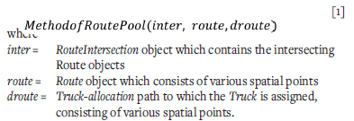
In TSJSim, the decision points are located with the spatial points on the Route objects, with each decision point at the Routelntersection having its own RoutePool list. A recursive algorithm which consists of three embedded for-loops and one defined function was developed for generating all the possible truck-allocation paths at the various decision points. The function, named MethodofRoutePool with the three input parameters, calls itself recursively to determine the RoutePool lists.

The starting point of the path is at the Routelntersection, and the ending point is at the Loader or the Dump or the next Routelntersection.

Figure 4 illustrates the flow chart for the algorithm. The main aim is to check all the nodes and the associated Route objects of the tree structure from the top to the bottom.

 

 

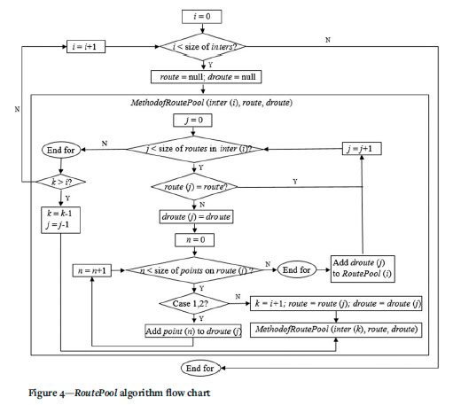
The outermost for-loop function loops through all the Routelntersection objects in the truck-shovel network system. For the ith Routelntersection object, i.e., inter (i), the MethodofRoutePool (inter, route, droute) is implemented to determine RoutePool (i), which is the RoutePool list at inter (i). The parameter route temporarily saves the Route object that was passed from the previous MethodofRoutePool function (if any), and the parameter droute temporarily saves the paths already generated by all the previous MethodofRoutePool functions (if any). For example, consider the RoutePool list at RouteIntersection A in Figure 2. Suppose the MethodofRoutePool function is used for RouteIntersection C. Then the current route parameter would be Route 2 and the current droute parameter would be the path A-B-C (Figure 3). The initial values of route and droute are set to null, since the starting point of the truck-allocation path at the Routelntersection contains no previous Route objects or paths (e.g., Node A in Figure 3). The MethodofRoutePool (inter, route, droute) has an inner for-loop function which loops through all the Route objects at inter (i), i.e., all the intersecting routes at the intersection. Within this for-loop, route (j) is compared with the route to check for new branches at the intersection. If route (j) and the route input parameter are two different Route objects, then a new truck-allocation path, i.e., droute (j), is initiated and replaced by droute. After that, the third for-loop function loops through all the points on Route (j) to check whether to add point (n) to droute (j) or to implement another MethodofRoutePool for inter (the next intersection). Depending on the location of point (n) on Route (j), the following three conditional statements are executed to control the recursion:

> If the decision point at inter (i) is connected with a destination, and point (n) is located between inter (i) and the destination, then point (n) is added to droute (j).

> If the decision point at inter (i) is connected with another decision point, and point (n) is located between inter (i) and inter on route (j), then point (n) is added to droute (j).

> If point (n) is the decision point at inter on route (j), then the MethodofRoutePool is implemented with inter (i+1), route (j) and droute (j) as the input parameters.

In the case where multiple decision points exist in the system, the spatial points between inter (i) and inter are first added to droute (j) at inter (i). Then the second MethodofRoutePool for the next decision point at inter (i+1) is implemented. This process continues until the last MethodofRoutePool function is implemented for the last decision point at the bottom of the tree structure. In the implementation of this last MethodofRoutePool, if the spatial points of the droute (j) are between the last decision point and the destination, then the droute (j) for the Route object at inter (size of inters -1), i.e, the last RouteIntersection object, is added to RoutePool (i). After that, the algorithm executes the second last MethodofRoutePool for inter (size of inters -2), i.e., the second last Routelntersection object. This process continues until the first MethodofRoutePool is executed, thus solving RoutePool (i) at inter (i) by examining all the decision points from the top to the bottom of the tree structure. By following the above recursive process, all the RoutePool lists of the RouteIntersection objects are generated.

Truck allocation strategy

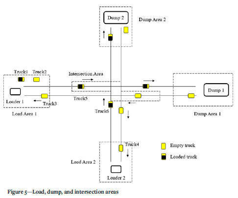
In TSJSim, the truck allocation decision is made by applying the multi-trucks-at-a-time approach, i.e., the trucks close to the decision points at the loading sites, dump sites, and traffic intersections are all considered in the truck allocation process. For modelling purposes, the truck-shovel haulage system is divided into the following three areas:

> Load Area is an area near the loader. Empty trucks haul toward the loader within this area. Trucks forming a queue at the loader and those trucks being loaded are all considered.

> Dump Area is an area near the dump. Loaded trucks haul towards the dump within this area. The queuing trucks at the dump and the trucks dumping are all considered.

> Intersection Area is an area near the intersection. Trucks hauling inside an intersection area and those trucks waiting outside the intersection area are all considered.

An example is shown, in Figure 5. When Truck 1 finishes loading and is ready for an assignment, in Load Area 1, Truck 2 is waiting, and Truck 3 is travelling empty to Loader 1. In Load Area 2, Truck 4 also travels empty to Loader 2. In the Intersection Area, Truck 5 is hauling a load to Dump 1 and Truck 6 is waiting outside the intersection area according to the passing priority rule (Zeng, Baafi, and Walker, 2019). These trucks are all close to the decision points. Hence Trucks 2, 3, 4, 5, and 6 as well as any other trucks that have already been assigned to respective dump sites could potentially influence the assignment of Truck 1 to a designated dump site.

 

 

Four truck-allocation strategies are developed as part of TSJSim model:

> Fixed truck assignment (FTA) - each truck is assigned to a fixed shovel and dump at all times. This truck-allocation rule serves as a baseline for comparing and evaluating the effectiveness of other truck-allocation strategies.

> Minimizing truck waiting time (MTWT) - the truck is assigned to the shovel or dump that is expected to generate the least amount of expected truck waiting time. The truck being loaded or dumping and the trucks in the queue are considered when estimating the total expected truck waiting time.

> Minimizing shovel production requirement (MSPR) - the shovels have predefined production targets and the trucks are assigned to the shovel with the maximum shortfall between the planned production and the ongoing simulated production.

> Minimizing truck semi-cycle time (MTSCT) - two optimization methods, i.e., the genetic algorithm (GA) and the frozen dispatching algorithm (FDA), were developed to implement MTSCT.

Definition of the truck semi-cycle time

One of the measures of the productivity and efficiency of a truckshovel mining system is the truck cycle time. In a complete truck cycle, the truck departs from a loader toward a dump site and then returns from this area back to a loader. The complete truck cycle time includes the loading time, hauling time from the loader to the dump site, queuing time at the dump site, dumping time, hauling time from the dump site to the same loading site or to another one, and queuing time at the loading site. One complete truck cycle includes two destinations:

> The departure destination, which is the planned destination of a truck when departing. If a truck is leaving a dump site, then a loading site would be the departure destination; if a truck is leaving a loading site, then a dump site would be the destination for the departing truck.

> The returning destination, which is the destination that a truck will return to after arriving at the departure destination. If a truck is leaving a dump site, then a dump site would be the destination for the returning truck. If a truck is leaving a loading site, then a loading site would be the destination.

Due to the influence of the ongoing truck allocations within the entire system, the further the truck travels, the more time the truck will spend on the route, and the more difficult it is to estimate the complete truck cycle time. The estimated queuing times at returning destinations vary more than those at departure destinations. If the complete truck cycle time is considered, the varying estimated queuing times at the return destinations may bias the truck allocation decision-making process for the departure destination.

In the TSJSim simulation model, a truck semi-cycle time is defined as the sum of the time durations for a truck travelling from the origin (i.e., a loader, dump or intersection) to its destination (i.e., a dump or loader site) plus the time for queuing and loading or dumping at the departure destination. The influence of the returning destination is not included in the truck semi-cycle time. The objective of the truck allocation algorithm is to obtain the assignment with the minimum estimated truck semi-cycle time.

Components of truck semi-cycle time

The estimated semi-cycle time for a truck at the decision point is expressed as:

where

et_ab = estimated semi-cycle time for a truck to travel from origin a, i.e., a loader, dump, or intersection, to destination b, i.e., a dump site or loading site

et_hb = estimated hauling time to arrive at destination b

et_qb = estimated initial queuing time at destination b

et_pb = estimated processing time (loading time or dumping time) at destination b

For the 'potential truck' close to a decision point, which is hauling to or waiting at a loader, dump, or intersection, the estimated semi-cycle time is:

where

et_ha = estimated hauling time to arrive at origin a, if the truck is still hauling et_qa = estimated initial queuing time at origin a, if the truck needs to queue

et_pa = estimated processing time (loading time or dumping time) at origin a

Suppose one truck just finishes dumping and is ready to be assigned to a loader. There could be n shovels in the network system, i.e., {s₁, s₂, s₃, ... , s_n} and m trucks that need to be allocated in this assignment, i.e., {t₁, t₂, t₃, ... , t_m}. The estimated semi-cycle time for each truck to reach the next decision point at a loader (when the truck finishes loading) can be expressed by Equation [4]:

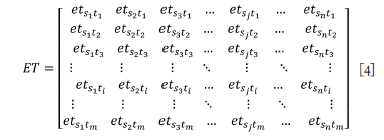
where

ET = matrix of estimated semi-cycle times for assigning m trucks to n shovels

et_sjt_i. = estimated semi-cycle time for truck t to arrive at shovel and to finish loading

If the estimated semi-cycle time of each truck is independent of all others, then the solution for t_i equals the minimum estimated semi-cycle time in {et_s1t_i, et_s2t_i, et_s3t_i,..., et_Snti}, i.e., min{et_s1t_i, et_s2ti, et_s3ti,..., et_snti}. However, the estimated semi-cycle times are not independent of one another because the trucks interact with each other in the truck-shovel mining network system. The interaction between the trucks includes the bunching effect on the haul route, the passing priority in the intersection area, and most importantly, queuing at the loader or dump site.

The estimated queuing time expressed in Equations [2] and [3] is an initial value which is the combined result of the present queue length at a loader or dump and the estimated hauling time. However, the actual estimated queuing time is not only influenced by the queue length, but also varies according to the truck-allocation. In TSJSim, optimization, methods were designed to change the estimated queuing time to reflect the influence of truck allocation decisions. As more trucks are assigned to the same loader or dump, the estimated queuing time increases, and the resultant increase in the estimated semi-cycle time is considered in the truck assignment.

Optimization methods for searching for the optimum destination with MTSCT

The genetic algorithm (GA) seeks the near-optimal solution by selecting the best solution and its neighbour, and then replacing the worst solution by the selected neighbour until the end of iterations (Gosavi, 2015). The general process structure of the GA is suitable for solving computationally complex problems (Alipour et al., 2017) and it has been used to tackle complex open-pit production scheduling problems due to its ability of producing near-optimal solutions within a short timeframe (Muke, Nhleko, and Musingwini, 2021).

In this paper, the GA and a newly designed algorithm based on the general structure of the GA, i.e, the frozen dispatching algorithm (FDA), were developed to solve the truck allocation problem, respectively.

Genetic algorithm (GA)

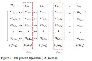
In TSJSim, the decision variables (Trucks) are stored in a list named truckListDV, {t₁, t₂, t₃, ... , t_m}, and their values or destinations, (at shovels or dump sites) are stored in a list named DVV, {s₁, s₂, s₃, ... , s_n}. The size of the solutionList is set to the number of destinations in the system, {SL₁, SL₂, SL₃,..., SL_j,...,SL_n}. A solution, SL_j, consists of m elements for all the decision variables. The element value is the estimated truck semi-cycle time:

where

SL_j = j^th solution, j e [1,n]

et_sjti. = estimated truck semi-cycle time t_i to destination point s_j, i g [1,m]

Let r denote the iteration number of the algorithm and r_max the maximum number of iterations to be performed. Set r = 1 and r_max = a constant value depending on the size of the model. There is no rule to determine an optimal iteration number and it is usually set by the permissible amount of computer time. The GA steps are as follows:

> Calculate the function value for each solution, i.e., f(SL_j), which is the accumulated estimated semi-cycle times for all the trucks. The steps for calculating f(SL_j) are as follows:

- Rank et_sjti. in SL_j in ascending order. In the new SL_j, t₁ will be the first truck to arrive at destination s_j, t₂ the second truck, and t_i the ith truck.

- Modify the estimated queuing time of each semi-cycle time element. When t_i arrives at s_j, if the shovel is still loading t_i-1, i.e., the expected arrival time of t_i is less than the expected departure time of t_i-1, then the queuing time is added to et_sjti.

- Sum all the modified semi-cycle time elements in SL_j, namely,

> Compare and rank SL_j in solutionList according to f(SLj). Denote the minimum by SL_min and the maximum by SL_max. Randomly select a neighbour of SL_min, and call it SL_nw, i.e., new = min + a random integer{-1,1}. Replace SL_max by SL_new, in other words, SL_max = SL_new. Referring to Figure 6, suppose SL_min is SL₂ and SL_max is SL₄. Initiate SL_new by reproducing SL_min, and then replace all the elements in SL_new with the elements in the neighbouring solution list. For instance, the replacement for et_S2ti can be either et_s1t1 or et_s3t1, depending on the generated random number.

 

 

> Increment r by 1. If r = r_max, return SL_min as the optimum solution and STOP. Otherwise, go back to step 1.

Frozen dispatching algorithm (FDA)

The FDA module was originally designed for the TSJSim model based on the actual behaviour of a truck-shovel mining system. The FDA's basic steps are summarized below:

> Select the element with a minimum value or element in list

ET_ti = {et_s1ti et_s2ti et_s3t1 - et_snti} i e and store the element(s) of which the destination is s_j in list ET_sj, j e [1,n]. For example in Figure 7, suppose et_S1ti. is the minimum element in ET_ti. = {et_s1t1 et_s2t1 et_s3t1 ... et_snt1}, and et_s1t2 is the minimum element in ET_t2 = {et_s1t2 et_s2t2 et_s3t2 ... et_snt2}. Then et_s1t2 stored in ET_s1. If et_s3t3 et_s2t1 is the minimum element in ET_t3 = {et_s1t3 et_s2t3 et_s3t3 ... et_snt3}, then et_s3t3 is stored in ET_s3.

 

 

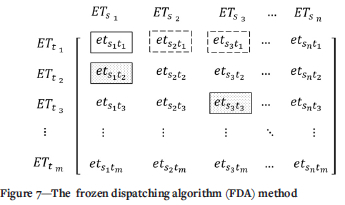
> Compare and rank the elements stored in ET_sj, j e [1, n]. If the minimum element in ET_S., j e [1, n], is et_sjtx, meaning the truck t_x is supposed to be the first truck to arrive at s_j and there will be no increase in queuing time for t_x at s_j, then the value of et_sjtx will not be changed. This assignment is 'frozen' and t_x will be assigned to s_j. For example, in Figure 7, the two elements, et_s1t1 and et_s1t2 in ET_s1, are compared and ranked. If et_s1t2 is the minimum element, then et_s1t2 is 'frozen' (shaded block) and t₂ will be assigned to s₁. ET_s3 contains only one element, et_s3t3. Thus, et_s3t3 is 'frozen' (shaded block) and t₃ will be assigned to s₃.

> Consider the elements in ET_Sj. j e [1, n], that are not 'frozen'. The truck with the minimum estimated time duration should arrive at the destination first and cause other 'unfrozen' trucks in ET_Sj. to wait on the condition that they arrive at the destination before the already assigned truck finishes loading or dumping. Therefore, the expected queuing time is added to other elements in ET_Sj.. To add the queuing time, first add the queuing time to the second minimum element (e.g., et_s1t1 in Figure 7) and then repeat steps 1 and 2. If:

- et_s1t1t is still the minimum element in ET_t1, this element would be 'frozen'.

- et_s2t1 is the minimum element in ET_t1, since it is the only element in ET_s2 , it would be 'frozen'.

- et_s3t1 is the minimum element in ET_t1, it would be compared with other 'unfrozen' elements in ET_s3 to decide whether it is the second minimum element in ET_s3^.

After the second minimum element is 'frozen', the third minimum element in ET_sj. is considered. This process continues until all the elements in ET_sj are all 'frozen'.

 

Comparison of truck allocation strategies

The following two sensitivity analyses were evaluated using the TSJSim model.

> The influence of the truck allocation strategies on the KPIs in the case where the truck-shovel matches varied.

> The influence of multiple truck-allocation decision points on the KPIs of the truck-shovel system.

Truck allocation strategies where the truck-shovel matches change

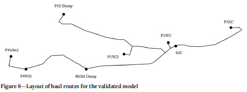
A simplified simulation model was established using TSJSim. This model was validated using field data collected by Shaw (2012) at a truck-shovel mining operation in Western Australia. The mining operation, known as Easter Ridge OB23/25, consists of four loading sites, named S4C, P3WC, P3EC, and P4, and four dumping sites, P1ED, P3WD, P4WD and ROM dump (Figure 8). The routes between P3WC, S4C, and the ROM dump were selected for this sensitivity analysis. The fleet in the system comprises Shovel 1 working at P3WC with associated trucks (named fleet 1, made up of CAT 785Cs) and Shovel 2 serving S4C with associated trucks (named fleet 2, made up of Komatsu 860Es). The main operational inputs are shown in Table I.

 

 

 

 

Four truck allocation strategies were considered. They are Fixed Truck Assignment (FTA), Minimizing Shovel Production Requirement (MSPR), Minimizing Truck Waiting Time (MTWT, and Minimizing Truck Semi-cycle Time (MTSCT), which included GA and FDA optimization. The simulation results included system production, truck queuing time, and bunching time.

The total fleet size varied from 10 to 19 so that the truckshovel match changed from both shovels under-trucked, to one shovel under-trucked and the other over-trucked, and then to both shovels over-trucked.

The assumptions for the model implementation are as follows:

> The trucks are not allowed to overtake each other along the routes

> The simulation model performs eight hours per shift during one simulation run, using a hot seat shift changeover, without considering other operational delays in the system

> Each design experiment is implemented with 100 simulation replications.

The simulation results are as follows.

System production tons

Figure 9 shows the relationship between the system shift production tons and the system fleet size using the four truck-allocation rules, i.e., MSPR, MTWT, GA, and FDA.

 

 

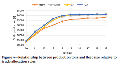
The MSPR, MTWT, GA, and FDA rules demonstrated similar increasing trends in shift production tonnages. Production using FDA remained higher compared with other rules. The trends can be divided into the following stages:

> Fleet size e [10,11]: When both Shovel 1 and Shovel 2 were under-trucked, as the fleet size increased from 10 to 11, the shift production tonnages increased.

> Fleet size e [12,16]: When Shovel 1 was under-trucked and Shovel 2 was over-trucked, as the fleet size increased from 12 to 14, the shift production tonnages continued to increase. When the total fleet size exceeded 14, i.e., six CAT 785Cs and eight Komatsu 860Es in the system, the shift production tonnages remained stable.

> Fleet size e [17,19]: When both Shovel 1 and Shovel 2 were over-trucked, all the shift production tonnages remained stable as the total fleet size increased from 17 to 19.

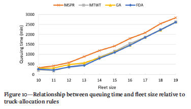
Queuing time

Figure 10 shows the trends of total queuing time (includes times at shovel and dump) versus the system fleet size using the truck allocation rules. The MSPR, MTWT, GA, and FDA rules all resulted in similar trends with respect to the queuing times. The queuing times showed a stable increasing trend as the fleet size increased. When the fleet size increased from 12 to 16 (when Shovel 1 is under-trucked and Shovel 2 is over-trucked), the queuing times had similar increasing rates as when fleet size increased from 17 to 19 (when both shovels are over-trucked). The queuing time using the FDA rule remained lower than queuing times generated using other rules.

 

 

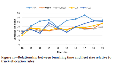
Bunching time

Figure 11 illustrates the trends of bunching times versus the fleet size using the truck allocation rules, ,., FTA, MSPR, MTWT, GA, and FDA. The bunching times using the MSPR, MTWT, GA. and FDA rules were all less than the bunching time when using the FTA rule, meaning that the bunching effect in the model was reduced when the truck allocation rules were applied.

 

 

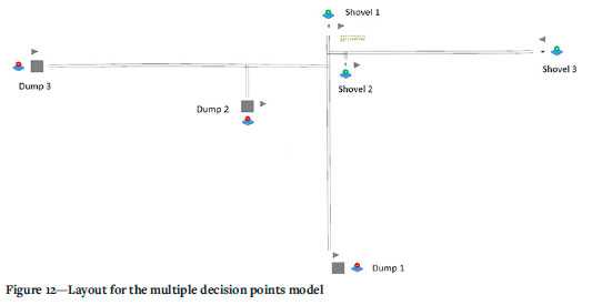
Multiple decision points effect

A truck-shovel haulage network system with multiple traffic intersections was constructed. Figure 12 illustrates the model layout, which consists of three loading areas, three dumps, and four traffic intersections along with the associated routes. There are 21 trucks (11 CAT 785Cs and 10 Komatsu 860Es) and three shovels of the same type in the system. The main operational inputs are shown in Table II .

 

 

Two cases were considered in the sensitivity analysis:

> Trucks were assigned only at loading areas and dumping areas and the decision points at traffic intersections were not considered.

> Trucks were also assigned at the decision points located at traffic intersections.

The Minimizing Shovel Production Requirement (MSPR), the Minimizing Truck Waiting Time (MTWT), and the Frozen Dispatching Algorithm (FDA) were considered for the sensitivity analysis. The simulation outputs included the system shift production tons and the total lost time, i.e., the sum of total queuing time and total bunching time.

Figure 13 illustrates the system shift production tons using the MSPR, MTWT, and FDA rules. If the decision points at the intersections were not considered, the system shift production tons using the MSPR, MTWT, and FDA rules were 63 114 t, 79 684 t, and 80 577 t, respectively. If the decision points at the intersections were considered, the system shift production tons using the MSPR, MTWT, and FDA rules increased to 70 196 t, 82 090 t, and 85940 t, respectively.

 

 

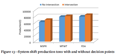
Figure 14 illustrates the total lost times using the MSPR, MTWT, and FDA rules. If the decision points at the intersections were not considered, the total lost time using the MSPR, MTWT and FDA rules was 3 271 minutes (54.5 hours), 2 147 minutes (35.8 hours), and 1 679 minutes (28.9 hours), respectively. If the decision points at the intersections were considered, the total lost time using the MSPR, MTWT, and FDA rules decreased to 2 781 minutes (46.4 hours), 1 513 minutes (25.2 hours), and 1 168 minutes (19.5 hours), respectively.

 

 

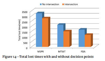
By considering the decision points at the intersections in the simulation model, both the system productivity and the fleet utilization significantly improve. According to the observation, the intersection decision points should be considered in the truck allocation decision-making process.

 

Conclusions

A realistic discrete event truck-shovel JaamSim simulator (TSJSim) was developed and integrated with the traffic module and the truck allocation module. The truck allocation module considers multi-trucks-at-a-time and multi-decision-points in the truck allocation strategy. The frozen dispatching algorithm and genetic algorithm were developed for the truck allocation optimization. The sensitivity analyses were designed and implemented based on the TSJSim simulation model. The inferences drawn from the truck-allocation evaluation models are summarized as follows.

> In the simulated truck-shovel system with two fleets: the changing trends for the production and queuing times utilizing the four truck-allocation strategies (MSPR, MTWT, FDA, and GA) all demonstrated similar patterns as the fleet size varied. As the system fleet size increased, the system production tons under these truck-allocation strategies at first increased significantly and then remained stable. The queuing time under these truck allocation strategies showed a positive relationship with the system fleet size. The bunching time decreased when the truck allocation strategies were applied in the model.

> In the simulated truck-shovel network system with multiple traffic intersections, both productivity and fleet utilization increased by assigning the trucks at the intersections. Thus, the multiple decision points along the haul routes should be considered in the truck allocation decision-making process.

Generally, the optimum fleet size for a truck-shovel system is determined using the MF (s) of the loader(s). Yet, when truck allocation strategies are applied, the number of trucks assigned to the loaders, the loader cycle times, and the truck cycle times may vary owing to flexible truck assignments. This issue is remedied with TSJSim, which can evaluate the influence of the truck allocation strategies on KPIs when the system fleet size is changed.

 

CRediT author statement

Weiguo Zeng: Conceptualization, Methodology, Software, Investigation, Validation, Formal analysis, Writing, Visualization; Ernest Baafi: Resources, Writing- Reviewing and Editing, Supervision, Project administration; Haiying Fan: Software, Investigation, Validation.

 

References

Afrapoli, A.M. and Askari-Nasab, H. 2017. Mining fleet management systems: A review of models and algorithms. International Journal of Surface Mining, Reclamation and Environment, vol. 33, no. 1. pp. 42-60. doi: 10.1080/17480930.2017.1336607        [ Links ]

Alarie, S. and Gamache, M. 2002. Overview of solution strategies used in truck dispatching systems for open pit mines. International Journal of Surface Mining, Reclamation and Environment, vol. 16, no. 1. pp. 59-76.         [ Links ]

Alipour, A., Khodaiari, A.A., Jafari, A., and Moghaddam, R.T. 2017. A genetic algorithm approach for open-pit mine production scheduling. International Journal of Mining and Geo-Engineering, vol. 1, no. 51. pp. 47-52.         [ Links ]

Askari-Nasab, H., Frimpong, S., and Szymanski, J. 2007. Modelling open pit dynamics using discrete simulation. International Journal of Surface Mining, Reclamation and Environment, vol. 21, no. 1. pp. 35-49.         [ Links ]

Baafi, E. Y. and Ataeepour, M. 1998. Using ARENA® to simulate truck-shovel operation. Mineral Resources Engineering, vol. 7, no. 3. pp. 253-266.         [ Links ]

Bonates, E. and Lizotte, Y. 1988. A computer simulation model to evaluate the effect of dispatching. International Journal of Surface Mining, Reclamation and Environment, vol. 2, no. 2. pp. 99-104.         [ Links ]

Dindarloo, S.R., Osanloo, M., and Frimpong, S. 2015. A stochastic simulation framework for truck and shovel selection and sizing in open pit mines. Journal of The Southern African Institute of Mining and Metallurgy, vol. 115, no. 3. pp. 209-219.         [ Links ]

Ebrahim, T., John, S., Virginia, I., and Danny, T. 2015. Simulation and animation model to boost mining efficiency and enviro-friendly in multi-pit operations, International Journal of Mining Science and Technology, vol. 25, no. 4. pp. 671-674.         [ Links ]

Elbrond, J. and Soumis, F. 1987. Towards integrated production planning and truck dispatching in open pit mines. International Journal of Surface Mining, Reclamation and Environment, vol. 1, no. 1. pp. 1-6.         [ Links ]

Fioroni, M.M., Franzese, L.A.G., Bianchi, T.J., Ezawa, L.R.P., and Miranda, G. 2008. Concurrent simulation and optimization models for mining planning. Proceedings of the 2008 Winter Simulation Conference, Miami, FL, 7-10 December 2008.. IEEE, New York. doi: 10.1109/WSC.2008.4736138        [ Links ]

Gosavi, A. 2015. Simulation-based Optimization: Parametric Optimization Techniques and Reinforcement Learning. Springer, New York.         [ Links ]

Gurgur, C.Z., Dagdelen, K., and Artittong, S. 2011. Optimisation of a real-time multi-period truck dispatching system in mining operations. International Journal of Applied Decision Sciences, vol. 4, no. 1. pp. 57-79.         [ Links ]

Hashemi, A. S. and Sattarvand, J. 2015. Simulation based investigation of different fleet management paradigms in open pit mines - A case study of Sungun copper mine. Archives of Mining Sciences, vol. 60, no. 1. pp. 195-208.         [ Links ]

Hauck, R.F. 1973. A real-time dispatching algorithm for maximizing open-pit mine production under processing and blending requirements. Proceedings of the Seminar on Scheduling in Mining, Smelting and Metallurgy, Montreal, Canada. CIM, Montreal.         [ Links ]

JaamSim. 2022. JaamSim software. http://jaamsim.com/ [accessed 1 April 2022].         [ Links ]

Jaoua, A., Gamache, M., and Riopel, D. 2012a. Specification of an intelligent simulation-based real time control architecture: Application to truck control system. Computers in Industry, vol. 63, no. 9. pp. 882-894.         [ Links ]

Jaoua, A., Riopel, D., and Gamache, M. 2012b. A simulation framework for realtime fleet management in internal transport systems. Simulation Modelling Practice and Theory, vol. 21, no. 1. pp. 78-90.         [ Links ]

Kolonja, B., Kalasky, D.R., and Mutmansky, J.M. 1993. Optimization of dispatching criteria for open-pit truck haulage system design using multiple comparisons with the best and common random numbers. Proceeding of the 1993 Winter Simulation Conference, Piscataway, NJ. IEEE, New York. pp. 393-401.         [ Links ]

Li, Z. 1990. A methodology for the optimum control of shovel and truck operations in open-pit mining. Mining Science and Technology, vol. 10, no. 3. pp. 337-340.         [ Links ]

Lizotte, Y. and Bonates, E. 1987. Truck and shovel dispatching rules assessment using simulation. Mining Science and Technology, vol. 5, no. 1. pp. 45-58.         [ Links ]

Mena, R., Enrico, Z., Fredy, K., and Adolfo, A. 2013. Availability-based simulation and optimization modeling framework for open-pit mine truck allocation under dynamic constraints. International Journal of Mining Science and Technology, vol. 23, no.1. pp. 113-119.         [ Links ]

Muke, P.M., Nhleko, A.S., and Musingwini, C. 2021. A genetic algorithm model for optimising long-term open-pit mine production scheduling. APCOM 2021.         [ Links ]

Proceedingsof Minerals Industry 4,0, 29 August 2 September. Southern African Institute of Mining and Metallurgy, Johannesburg.         [ Links ]

Ouelhadj, D. and Petrovic, S. 2009. A survey of dynamic scheduling in manufacturing systems. Journal of Scheduling, vol. 12, no. 4. pp. 417-431.         [ Links ]

Pfeiffer, A., Kadar, B., and Monostori, L. 2007. Stability-oriented evaluation of rescheduling strategies, by using simulation. Computers in Industry, vol. 58, no. 7. pp. 630-643.         [ Links ]

Que, S., Anani, A., and Awuah-Offei, K. 2016. Effect of ignoring input correlation on truck-shovel simulation. International Journal of Mining, Reclamation and Environment, vol. 30, no. 5-6. pp. 405-421.         [ Links ]

Shaw, G. 2012. Proactive production estimation and fleet management of a surface mining operation. BE (Mining) thesis, University of Wollongong.         [ Links ]

Sofranko, M., Wittenberger, G., and Skvarekova, E. 2015. Optimisation of technological transport in quarries using application software. International Journal of Mining and Mineral Engineering, vol. 6. pp. 1-13.         [ Links ]

Soumis, F., Ethier, J., and Elbrond, J. 1990. Evaluation of the new truck dispatching in open pit mines. Proceedings of the 21st International Symposium on the Application of Computers and Operations Research In the Minerals Industry. pp. 674-682.         [ Links ]

Ta, C.H., Kresta, J.V., Forbes, J.F., and Marquez, H.J. 2005. A stochastic optimization approach to mine truck allocation. International Journal of Surface Mining, Reclamation and Environment, vol. 19, no. 3. pp. 162-175.         [ Links ]

Ta, C.H., Ingolfsson, A., and Doucette, J. 2013. A linear model for surface mining haul truck allocation incorporating shovel idle probabilities. European Journal of Operational Research, vol. 231, no. 3. pp. 770-778.         [ Links ]

Temeng, V.A. 1997. A computerized model for truck dispatching in open pit mines. PhD thesis, Michigan Technological University.         [ Links ]

Upadhyay, S.P. and Askari-Nasab, H. 2017. Dynamic shovel allocation approach to short-term production planning in open-pit mines. International Journal of Mining, Reclamation and Environment, vol. 33, no. 1. pp. 1-20. doi: 10.1080/17480930.2017.1315524        [ Links ]

White, J.W. and Olson, J.P. 1986. Computer-based dispatching in mines with concurrent operating objectives. Mining Engineering, vol. 38, no.11. pp. 1045-1054.         [ Links ]

White, J. W. and Olson, J.P. 1993. On improving truck/shovel productivity in open pit mines. CIM Bulletin, vol. 86, no. 973. pp. 43-49.         [ Links ]

Wu, K. and Garcîa de Soto, B. 2020. Spatiotemporal modelling of lifting task scheduling for tower cranes with a tabu search and 4-D simulation. Frontiers in Built Environment, vol. 6, no. 79. doi: 10.3389/fbuil.2020.00079        [ Links ]

Yilmaz, E. and Erkayaoglu, M. 2021. A discrete event simulation and data-based framework for equipment performance evaluation in underground coal mining. Mining, Metallurgy & Exploration, vol. 38. pp. 1877-1891.         [ Links ]

Zeng, W., Baafi, E.Y., Walker, D., and Cai, D. 2016. A 3D discrete event simulation model of a truck-shovel network system. Proceedings of the Ninth AUSIMM Open Pit Operators' Conference, Kalgoorlie, Australia. Australasian Institute of Mining and Metallurgy, Melbourne. pp. 265-273.         [ Links ]

Zeng, W., Baafi, E.Y., and Walker, D. 2019. A simulation model to study bunching effect of a truck-shovel system. International Journal of Mining, Reclamation and Environment, vol. 33, no. 2. pp. 1-16. doi: 10.1080/17480930.2017.1348284        [ Links ]

 

 

Correspondence:
W. Zeng
Email: wz999@uowmail.edu.au

Received: 30 Apr. 2022
Revised: 8 Oct. 2022
Accepted: 18 Oct. 2022
Published: December 2022