


Services on Demand
Article
 English (pdf)
 Article in xml format
 Article references
Indicators

Related links
-
 Cited by Google
 -
 Similars in Google
Share

 Permalink
Journal of the Southern African Institute of Mining and Metallurgy
On-line version ISSN 2411-9717
Print version ISSN 2225-6253
J. S. Afr. Inst. Min. Metall. vol.122 n.12 Johannesburg Dec. 2022
http://dx.doi.org/10.17159/2411-9717/1036/2022
PROFESSIONAL TECHNNICAL AND SCIENTIFIC PAPERS
Stochastic analysis of dig limit optimization using simulated annealing
J.R. van Duijvenbode; M.S. Shishvan
Resource Engineering, Department of Geosciences and Engineering, Delft University of Technology, Netherlands. ORCID: J.R. van Duijvenbode: https://orcid.org/0000-0001-6723-0167; M. Soleymani: https://orcid.org/0000-0002-0780-8841
SYNOPSIS
The results of dig limit delineation in open pit mining are never truly optimized due to gaps in the underlying data, such as insufficient sampling. Aside from the data uncertainty, there is also an influence on the final dig limit by either humans or by the heuristic character of an optimization method like simulated annealing. Several dig limit optimizers have been published, which can replace the manual dig-limits designing process. However, these dig limit designs are generally not adapted to account for this heuristic character. In this paper we present a stochastic analysis tool that can be used with the results of heuristic dig-limit optimization to increase confidence in the obtained results. First, an enhanced simulated annealing algorithm for dig limit optimization is presented. Then, this algorithm is tested on ten different blasts at the Marigold mine, Nevada, USA, as a case study. Finally, the results are analysed with a destination-based ensemble probability map and an analysis conducted of the final solution data distribution. The generated dig-limit designs of the algorithm include high revenue areas that are excluded in comparable manual designs and show improved objective and revenue values. The analysis tool provides block destination probabilities and box plots with the distribution of opportunity value for the dig limit. Furthermore, with the analysis tool, it is possible to make well-informed design decisions in areas of uncertainty.
Keywords: open-pit mining, dig-limit optimization, simulated annealing, grade control.
Introduction
Hard rock open-pit mining involves the blasting of mining benches, after which the blasted material is sent to an assigned destination. Making decisions concerning the different material types from a bench and their destinations is commonly known as grade control (Dimitrakopoulos and Godoy, 2014; Kumral, 2013; Verly, 2005). Grade control often relies on the results of grade analysis from blast-hole sampling (or dedicated grade control sampling). Modelling the spatial distribution of these grades results in a high-resolution grade control model, which helps with assigning an appropriate destination to a group of blocks. This approach, known as dig -limit delineation, aims to correctly cluster a group of blocks, which should be mineable, and outline and separate various ore types and waste material (Richmond and Beasley, 2004).
Recently various researchers have developed algorithms to automate and optimize the dig limit delineation process, which rely on heuristics and metaheuristic algorithms. The techniques used include greedy algorithm-based methods (Richmond and Beasley, 2004; Vasylchuk and Deutsch, 2019), mixed integer programming (MIP) (Hmoud and Kumral, 2022; Nelis and Morales, 2021; Nelis, and Meunier, 2022; Sari and Kumral, 2017; Tabesh and Askari-Nasab, 2011), genetic algorithms (Ruiseco, 2016; Ruiseco, Williams, and Kumral, 2016; Ruiseco and Kumral, 2017; Williams et al., 2021), simulated annealing (Deutsch, 2017; Hanemaaijer, 2018; Isaaks, Treloar, and Elenbaas 2014; Kumral, 2013; Neufeld, Norrena, and Deutsch, 2003; Norrena and Deutsch, 2001), block aggregation by clustering (Salman et al., 2021) and convolutional neural networks (Williams et al., 2021), or a combination of techniques. With these algorithms, the definition of 'mineability' or 'digability' varied greatly between different investigators. The mineability of a dig limit is a quantitative measure that expresses how well a given item of equipment can extract the material without incurring dilution or ore loss. Earlier research methodologies used polygons and circles for dig limit designs (e.g., Neufeld, Norrena, and Deutsch, 2003), whereas currently blocks are often considered.
An example of a greedy dig-limit delineation algorithm can be found in Richmond and Beasley (2004). They used a floating circle-based perturbation mechanism to satisfy the mining equipment constraints. To delineate ore zones, the method uses a floating circle, which moves over the grade control model and expands until the average grade of the covered blocks is below the cut-off grade. This process is repeated multiple times, and the results are stored and evaluated by a mean-downside risk efficiency model that evaluates their dig limit solutions considering the financial risk for the dig limit design. Wilde and Deutsch (2007) used a feasibility grade control (FGC) method to optimize the dig limit profit, which iteratively recalculates the objective value by amalgamating blocks into mining units. Two constraints applied to the mining unit are that all blocks must have an adjacent block with the same destination, and the shape must be easily extractable. Vasylchuk and Deutsch (2019) used a method where dig limits are subject to site-specific rectangular excavating constraints. To satisfy the constraint, the method uses a floating (rectangular) frame that moves over the grade control model. The frame was analysed for its optimal destination, and this destination was assigned to the blocks. Finally, their model adapted problematic locations by reconsidering the neighbouring blocks and their destinations and performed a hill climbing step to improve the solution iteratively. Williams et al. (2021) recently explored GA solutions using a CNN to assess the dig limit cluster quality. The algorithm was very fast but could not well distinguish different clustering penalties (position- and-orientation-related).
More frequently applied optimization methods for solving dig limit problems include SA, GA, and MIP. SA is a metaheuristic, stochastic search algorithm used to approximate the global optimum of a given function (Aarts, Korst, and van Laarhoven, 1997; Kirkpatrick, Gelatt, and Vecchi, 1983; Rutenbar, 1989). The algorithm moves towards a final (optimum) solution by accepting or rejecting solutions based on an acceptance probability (Kirkpatrick, Gelatt, and Vecchi, 1983). SA has been used widely in the mining industry for various optimization problems, for example, for resource modelling (Deutsch, 1992), optimization of blasting costs (Bakhshandeh Amnieh et al., 2019), strategic open-pit mine production scheduling (Dimitrakopoulos, 2011; Kumral and Dowd, 2005) for multiple destinations (Jamshidi and Osanloo, 2018) with and without stockpile considerations (Danish et al., 2021) or blast movements (Hmoud and Kumral, 2022). These applications focus on maximizing the profit for mining of each mining block by considering revenues, penalties, dilution factors, or mining constraints. Typically, the results are used in short-term planning, as input for blast design or grade control, surveying, and for field markup of mining benches (Maptek Vulcan, 2016).
In this paper we focus on the application of SA to the dig limit problem, as in Isaaks, Treloar, and Elenbaas (2014) and Hanemaaijer (2018). They used an optimization function that minimizes revenue loss due to wrong block assignments but limited their outcomes to only one near-optimal solution. Their constraints focused explicitly on creating dig limits that account for equipment constraints. For this constraint, they assigned a minimal mining width (MMW) that prevented the individual selection of blocks. Similarly, Ruiseco (2016) and Ruiseco and Kumral (2017) used a GA algorithm for the dig limit selection problem. In addition, they assigned a penalty, when blocks deviated from the correct clustering size. The correct clustering size is related to the mineability and how well a block of material can be extracted. Finally, the algorithm accepted a final solution with the highest objective value. Ruiseco's work also showed a distribution from the solution's objective value after multiple runs and indicated the reliability of this non-optimal solution method. Sari and Kumral (2017) indicated that the dig limit selection problem was not solved using an exact method and therefore used MIP. Their approach complies with an MMW constraint by ensuring each block is connected to an ore or waste zone at least as big as the MMW.
Various commercial implementations of dig limit or grade control-related optimizers are available, which provide polygon outlines as a result (Deswik, 2019; Isaaks, Treloar, and Elenbaas, 2014, Maptek Vulcan, 2016; Orica, 2021). However, only from the mineable shape optimization tool, it is known that it uses a SA and/or a branch and bound algorithm (Deutsch, 2017; Maptek Vulcan, 2016). Furthermore, these applications have limited flexibility and provide few insight into details of the algorithms for solving the dig limit optimization problem, or the probability or quality of any of the solutions. This substantiates the need for an improved SA application methodology which runs multiple dig-limit optimizations and gives a stochastic probability insight into the quality of the solutions.
In this paper we investigate the stochasticity of dig limit optimization through SA using an enhanced framework that uses similar frame and MMW constraint ideas as mentioned above. However, the heuristic character of SA implies that the final solution could vary for each realiztion and motivates the use of multiple dig-limit realizations to reduce algorithm uncertainty and increase confidence in the results. The work does not use an interpolated (kriged) grade control model to better show the stochastic influences of dig limit optimization rather than stochastic influences by interpolation. This is also supported by the continuity of the case study orebody and spatially dense data-set of grades due to the small spacing between blast-holes. The SA algorithm is tested on a case study with ten blasts and dig limit designs. We explore the stochastic and metaheuristic effects of SA and dig limit optimization and describe a new tool for making conclusions regarding the dig limit design. The paper concludes with a discussion of the stochastic analysis tool and potential improvements.
Methodology
The following steps were performed to prepare the data-set for the SA algorithm, summarized in Figure 1a. First, a regular grid was fitted to the blast-holes that best represent these original data-points. The blast-hole coordinates were snapped onto the nearest point in this regular east-north grid. As mentioned, the approach's rationale was to avoid the commonly used kriging method because the initial assumption was that the blast-holes were planned at an (almost) regular densely spaced pattern, and y a high-resolution spatial model is not necessary as long as the average grade of the dig block can be estimated correctly. Finally, the assay results from multiple blast-holes were averaged to determine the metal grades at the grouped blast-holes. At this stage, the data-set was represented by regularized blast-holes with their corresponding attributes. It should be noted that no vertical dimension was used, as the assay results were averaged over the entire blast-hole, which removes the vertical dimension. No blast movement adjustments were made.
The following two concepts were used in the SA algorithm:
> Frames (Figure 1b) indicate the area around a blast-hole (node) that must comply with the MMW. Each blast is divided into frames that contain fx x fy number of nodes, where fx,fy are the frame dimensions in the east and north direction, respectively. Thus, for each node fx x fy possible frames exist.
> A misfit value is assigned when the destination of a node is not optimal in relation to the surrounding area, as shown in Figure 1c. The misfit value is defined as the number of nodes in any possible frame not assigned to the same destination as the largest group of nodes in the frame. It is independent of the destination of the misfits, and the value only indicates how many blocks in the frame are not sent to the largest destination group (Hanemaaijer, 2018). Objectives 2 and 3 from the objective function explain how the algorithm uses a node and frame misfit value to indicate the solution quality.
Simulated annealing framework
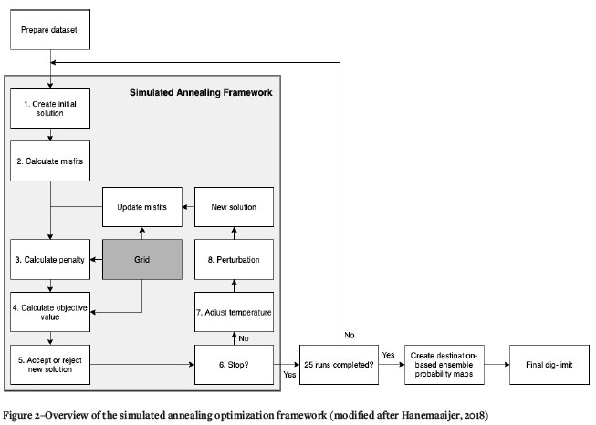
The presented algorithm uses all the steps of a normal SA algorithm (Kirkpatrick,Gelatt, and Vecchi 1983) to find an optimized solution regarding dig limit shape and revenue by minimizing switching between ore and waste and minimizing the MMW penalty. Normally, the solution is not guaranteed to be the optimal one, especially not during the first run and, therefore, it is proposed to run multiple SA optimizations and define a destination-based ensemble average for the dig limit. The SA framework (Figure 2) was previously described by Hanemaaijer (2018), but is adapted for this study to also produce the ensemble average maps. The algorithm is initialized with a dig limit design (initial solution) and maximized towards a final optimum by iterating over the following steps: penalty calculation, objective value calculation, accept/reject decision, temperature adjustment, perturbation of the solution, and stop criteria check. For each step of the algorithm, different variations were tested before the algorithm as presented was chosen. The reader is referred to Hanemaaijer (2018) and Villalba Matamoros and Kumral (2018) for more details. Each step of the SA framework (Figure 2) is explained in the following sections.
Initial solution
The SA algorithm automatically generates an initial solution from the regularized node data-set. For each non-overlapping frame, the best destination was chosen by determining the revenues for the nodes in the frame by setting all destinations to ore or waste. The highest revenue value determined the initial destination for the nodes in the frame. This procedure also accounted for frames that occurred at bench boundaries. Tests with a free selection or random initial solution provided similar results but entailed a longer computation time.
Objective function
The dig limit delineation problem is expressed as a maximization problem of the revenue by assigning the best destination to each node (a grade control block) and penalizing it due to constraint violations. Penalty weights are used to balance the importance and effect of the corresponding constraint on the dig limit design. The problem is solved by a multi-objective SA function, which consists of three components:
1. Maximize the blast revenue
2. Minimize witching between material types (frame misfit
3. Minimize the MMW penalty (minimal node misfit).
The objective function that determines the objective value is:
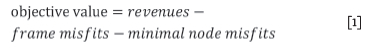
Objective 1. Selecting the right node destination will increase the revenue from extraction. If the ore is sent to the waste dump, there is opportunity loss, but when waste is classified as ore, the extra processing costs outweigh the value recovered. The objective, to get high revenue for a blast, is expressed as follows:
Maximize
where
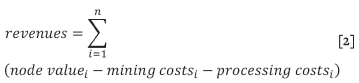
where n is the total number of nodes and i the index number of each node (i=1,...,n). Each i also represents a unique ix and iy position of the node along the corresponding axis (x=i,...,nx and y=i,...,ny), where nx and ny are the number of nodes in the east and north directions, p is the metal price, ri the recovery related to node i, g is the metal grade for node i, desti is the destination indication for node i, which is generally ore or waste, and mcwaste,mcore, and pcore are the mining and processing costs for waste and ore, respectively. No node mass was used in the optimization algorithm.
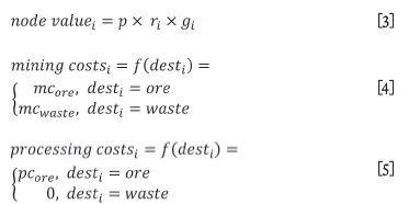
Objective 2. A frame misfit value is assigned to all possible frames in the blast grid (Figure 1c). Minimizing the frame misfit values helps the algorithm with the discouragement of switching between destinations. This is done with a higher frame misfit value which occurs when there are boundaries between destinations. This objective is defined as:
Minimize
where
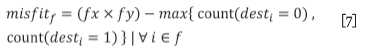
where fn is the total number of frames in the grid and f the index number of each frame (f=1,...fn), misfitf is the misfit value from frame f, fx and fy are the frame dimensions in the east and north directions, and max is the value of the largest group of node destinations in the frame (Figure 1c), wpF is the frame penalty weight. A high wpF will discourage frequent destination switching in a frame and results in bigger zones of one destination. However, a poorly selected value would result in too much ore loss and dilution.
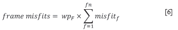
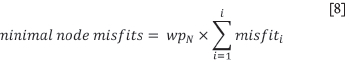
Objective 3. A node misfit is assigned to each node of the blast grid (Figure 1c). The node misfit is the minimum of all frame misfits from the frames that contain the given node. This misfit value helps to indicate whether a node is in at least one frame where all destinations are the same. Satisfying this ensures compliance with the MMW constraint of the equipment. This objective is expressed as:
Minimize
where
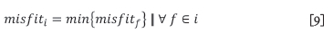
where misfiti is the misfit value from node i, min{misfitf} is the value of the smallest frame misfit value from all frames where the node corresponds to (Figure 1c), and wpN is the node penalty weight. Similar to the frame penalty weight, the value of wpN should be carefully selected. A small value will result in a highly selective dig-limit design, which is an infeasible solution.
Perturbation mechanism
The perturbation step generates new solutions by changing the destination of the nodes in one frame to a randomly chosen destination. The frame choice was either by selecting a frame with a misfitf > 0 or by a random frame. The first selection method helps to specifically induce changes at locations in the grid that have boundaries (for instance, a single waste node in an ore region). After perturbation, the minimal node and frame misfits were updated to accommodate the changes in node destination.
Acceptance criterion
The model uses a metropolis algorithm in order to have a stochastic criterion of acceptance of worse solutions. The Boltzmann probability P(accept)=e-dE/T defines the probability of acceptance of a worse solution, where dE is the absolute objective value difference between the new and old solution and T is the current temperature. The temperature is analogous with the model progress (cooling down). When the model cools down (progresses), then the changes in solutions become less sporadic. If the Boltzmann probability is greater than a random number between o and 1, then the new solution is accepted as the current solution and becomes the old solution. Conversely, if the probability is less than the random number, the algorithm rejects the new solution, and the old solution stays the same for comparison in the next iteration (Martín and Sierra, 2009).
Temperature decrement and termination rule
An epoch is a state of the algorithm where the temperature variable is not changed over a fixed number of iterations. After each epoch, the system cools by a quadratic additive cooling function which uses the total number of epochs and fixed final temperature:
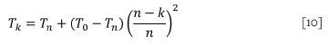
where Tk is the temperature at epoch number k, T0 the initial temperature, Tn the final temperature, and n the total cooling epochs (Martín and Sierra, 2009). The initial temperature ensures an initial acceptance ratio of approximately 0.5 and that the advantage of having a guided initial solution remains. When the system temperature reached Tn, it was kept running until the predefined total number of epochs, which was one of the stop criteria. The second stop criterion stops the algorithm earlier when a certain number of non-improving consecutive perturbations (iterations) is reached. This number was chosen to be greater than the total number of nodes in the grid, to ensure that at least every node could be randomly assigned once for perturbation.
Hanemaaijer (2018) tested four different temperature schedules, from which the quadratic additive cooling function was selected as the preferred function. It counteracts the exponential decay (see the Boltzmann probability) in the acceptance criterion with decreasing temperatures. This ensures that no major worse solutions are accepted any more (relatively fast), and that the cooling schedule, or Tn, becomes the termination criterion of the SA algorithm. Furthermore, it is fairly unlikely that new solutions will be found if Tn is reached and thus the choice of cooling function and speed has a direct bearing on the near-optimality of the SA.
Marigold mine case study
A case study was carried out to demonstrate the performance of the proposed SA algorithm for dig limit optimization. Two benches (A and- B), with five different blasts on each, were studied (Figure 3).

The Marigold mine (MG), in northern Nevada, USA, is owned and operated by Marigold Mining Company, a wholly owned subsidiary of SSR Mining Inc. A typical drill and blast, truck and shovel technique is used to extract the ore from several open pits. The ore is processed using heap leaching. An ore bench has a height of 7.6 m (25 ft) or 15.2 m (50 ft). The blast patterns are 7.3 m by 6.4 m for the waste benches and 7.6 m by 6.7 m for ore benches. The mine uses three shovels (2 x 28.7 m3 and 1 x 52.8 m3 bucket capacity), and the bucket widths define the typical minimal mining width (MMW) of 12.2-15.2 m or two blast-holes. Blast-hole sampling is done to define ore zones. One sample per blast-hole is assayed for gold in an on-site laboratory to obtain a cyanide-soluble and a fire-assay grade, which together determine the total gold value (Aui) contained in each blast-hole (Marigold Mine, 2017).
The traditional dig limit procedure involves entering fire equivalent grades associated with each blast-hole into the grade control model. The blast pattern is then converted to a new block model with block sizes of 3.05 m x 3.05 m x 7.6 m. Next, the blast-hole assay data is kriged using ordinary kriging in two dimensions on the bench. If there are enough blocks above the cut-off grade to constitute a mineable body of ore, this is manually blocked out and marked in the pit to be sent to the leach pad for processing (Marigold Mine, 2017). The data-set used in this paper was obtained in the way described above, except that the data was not kriged.
Design and parameter selection
The selected SA parameters were chosen after testing and parameter tuning (Table I), following procedures similar to those described by Hanemaaijer (2018). Table II displays th case study parameters corresponding with the MG operation. The algorithm is written in the Python programming language according to established geostatistical conventions (GSLIB convention), for example, with the east direction as the x-axis and the north direction as the y-axis (Deutsch and Journel, 1997).
Results
Objective value
For each of the ten blasts, 25 SA runs were conducted to perform a stochastic analysis on dig limit optimization using SA. Each run reached 1500 consecutive non-improving perturbations and caused the algorithm to stop. This shows that each run is converged to an optimum. The average run time was 160 seconds. For example, Figure 4 shows two solutions from level B blast 3, one with the highest objective value (a) and one with the highest revenue (b) from the 25 runs. The difference can be found in the lower left corner, where solution (a) selected a larger ore region. This raised the objective value by 0.57% because a lower penalty was assigned due to the switching between material types. The revenue difference between the two solutions is only 0.58%.
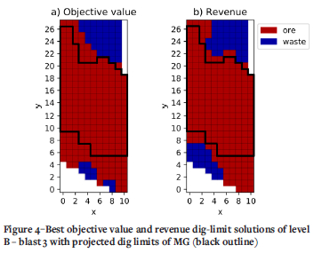
The black outlined area in Figure 4 indicates the ore zone from MG's dig limit solution. There is a big difference in the selected number of blocks and the associated loss in objective value and revenue. A 16% higher objective value and 5% higher revenue were found compared to MG's solutions. However, the solutions do not always comply with the MMW constraint (Figure 4a at node (6,1)). In these cases, the penalty for not complying with the constraint was lower than the benefit gained while complying. The penalty weights, wpF and wpN, were chosen such that destination switching was discouraged and the algorithm was forced to comply with the mining constraints (Hanemaaijer, 2018). That the outcome in terms of objective value (and revenue) is better than the manually created dig limit design is promising, despite the fact that SA does not guarantee optimality.
Revenue
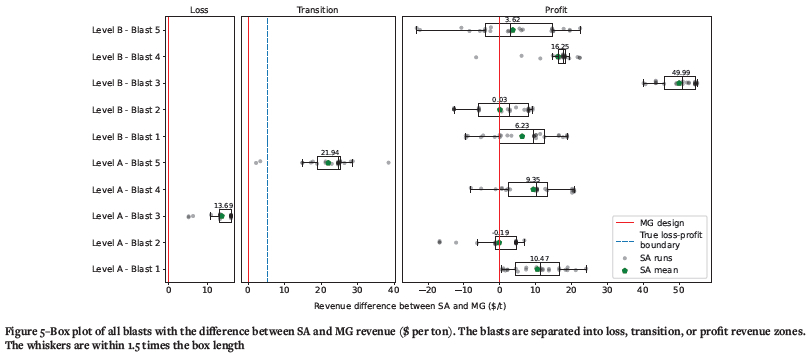
The revenues corresponding with the objective values were compared with the manual designed dig limit solutions from MG. Comparing the revenues could be misleading since optimization was done regarding the objective value. However, revenue is still one of the most important factors for the mine. The revenue differences between the MG dig limit and all blast optimization runs (25 each) are shown as box plots in Figure 5. The box extends from the lower to upper quartile values of the data, with a line at the median and the length of the whiskers being within 1.5 times the box length. The algorithm shows that it can improve revenue compared to the MG solution from mining the bench, whether it is in the loss, transition, or profit revenue zone. The boundary between the profit and loss revenue zones is where the total bench revenue moves from positive to negative. Generally, the loss zone corresponds with mining a lot of waste material (level A - blast 3). An improved dig limit reduces the mining costs, and less potential value ends up at the waste pile. Within the revenue transition zone, a potential loss is converted to a profit (dotted loss-profit boundary). It can be concluded that improvements in the profit region are beneficial for the mining company because small details could be improved during the manual designing process.
In nine out of ten cases the SA's mean was higher than the MG dig limit revenue (Figure 5). This indicates that the SA optimization performed well. The set of solutions with a small revenue improvement, in the range up to $15 per ton, suggests that MG's dig -limit solution was already reasonably good. Two solutions outperformed the MG solution with a difference of $22 and $50 per ton, respectively (level A - blast 5 and level B - blast 3). In these cases, the solution missed or included one or several regions rich in ore or waste. Finally, there was one solution that, on average, did not lead to any improvement (lA - blast 2). The main reason for this was that the grid preparation tool had difficulties in constructing the grid correctly. However, it is promising that better revenue solutions were found, and thus future improvements may also improve these difficult blasts.
Stochastic analysis
SA is a metaheuristic optimization method whereby accepting a solution does not guarantee an optimized result. Therefore, we analysed the probabilistic chance for achieving a good solution. Generally, the best solution from the solution distribution should be selected as the final solution. However, the quality of this solution depends on the number of runs. Increasing the number of runs costs more in computational time while not always giving a better result. An alternative consideration is to use a destination-based ensemble probability map which shows the areas the algorithm is struggling with.
Destination-based ensemble average
Figure 6 shows a revenue box plot and node (mining blocks) destination probability map for 25 SA runs of level A - blasts 1 and 5. The displayed node destination is the destination's ensemble average from the 25 runs. This ensemble average can be linked with the confidence of the algorithm and the probability that a node should be assigned to a destination. For instance, nodes with a destination probability of approximately 0.5 indicate uncertainty regarding the best destination of the node. Therefore, a single run from the algorithm could be misleading and insufficient.
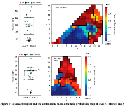
When a node's destination probability is higher, it suggests that this node causes the objective value to increase because the node reduces ore loss and dilution. Ore loss is decreased when nodes of good grade are inside the dig limit, and dilution is reduced when waste material is removed from the dig-limit. However, depending on the economics, it can be worthwhile to include a few waste nodes so that the dig limit can include a higher-grade ore node.
For example, if for a node with a destination probability of approximately 0.5 from level A - blast 1 it was decided to designate the material as waste, then no additional dilution and revenue was created. Thus, most likely, the revenue value of the resulting solution will be in the 25-50% quartile. Two additional factors should be considered when this node is designated as ore. First, when this node is included in the dig limit there is potential that the solution's revenue will increase due to reduced ore loss. Probably, the final solution's revenue will be in the 50-75% quartile. Conversely, the node can also be of low grade, causing the mining constraints to fail, including dilution, and reducing the revenue value. In addition, analysing the quartile ranges suggests that the potential revenue gain is smaller than the potential loss. Secondly, assigning this node as ore implies a neighbouring higher-grade ore node that is worthwhile to include in the dig limit. It should be checked whether this is applicable. For level A - blast 5, the 0.5 destination probability node (lower-right) can be better designated as waste since the added revenue value is relatively small. Additionally, selecting this node as waste ensures that the remaining dig limit is less diluted. Similar considerations could be made for the other blasts.
Distribution of final solution data
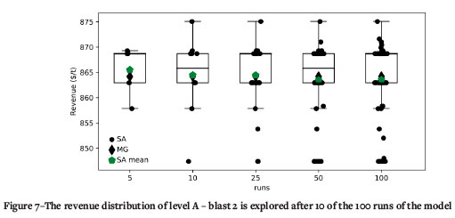
Analysing the variance of the objective value or revenue from all found solutions could be a measure for the final dig limit acceptance and how close the outcome of SA is to optimality. Hereby, no distinction is made whether the objective value or revenue distribution is considered. While doing multiple runs, an objective value or revenue boxplot could show the distribution of the final solution data at that moment. When enough of the solution space is explored, one approach is to accept the solution with the highest objective value at that moment and to consider the destination-based ensemble probability map. For example, Figure 7 displays the revenue distribution of 5, 10, 25, 50, and 100 consecutive runs for level A - blast 2. For this example, monitoring the data distribution change could already suggest that after ten runs, enough of the solution space is explored and that the corresponding highest objective value solution should be accepted as the final dig limit.
Analysing the revenue box plot while conducting multiple runs together with the associated destination-based ensemble average helps to inform a final decision regarding the dig limit design. The highest objective value solution provides the so-far best result, and the ensemble average gives more insight into potential interesting areas, which could be included in a final dig limit design.
It is known that the SA solutions are not guaranteed to be the global optimal solutions and they are optimized in terms of objective value and not revenue. However, from the distribution of solutions in Figure 7 and the associated objective values it is possible to estimate how close most of the solutions are to optimality in terms of objective value. The highest revenue solution ($875 per ton) was only found once (1% chance), but did not have the highest objective value due to its higher penalty. In contrast, the solutions with the highest objective value had a revenue of $863 per ton and would, therefore, better represent the near-optimal solution. The significant effect of the applied penalties is shown in the 100-run box plot in Figure 7 because most solutions are grouped at a revenue of $863 per ton (28 runs) and $869 per ton (45 runs). That implies that the highest revenue is not the global optimal solution, but that it is more likely to be related to the 73 solutions with a revenue between $863 and $869 per ton.
Discussion
The dig limit analysis tool gives insight into the existing variability of the dig limit results. This variability is due to the stochastic influences from the metaheuristic optimization method of simulated annealing. As opposed to using a single result, the destination-based ensemble averages and box plots were combined as a new data-set to show these stochastic influences. A sequential manual decision could directly incorporate this stochasticity into a final dig limit design. The destination-based ensemble average approach can also be used for dig limit results derived from GA or CNN approaches. These algorithms also provide near-optimal solutions, and running them multiple times will similarly give a distribution of opportunity values and designs for the dig limit. However, these approaches require a large population of solutions, for all of which the objective value needs to be evaluated. This makes SA easier to implement and less computationally intensive. The approach would not work for MIP because this will always give the same optimal solution if the problem is feasible. The computation time of the algorithm is also much longer than SA, GA, or CNN and likely not practical for real mining operations.
Normally, uncertainty in grade control is due to unknown (or interpolated) grades and to-be-included mining constraints. For example, for the areas with much uncertainty, the final (manual) destination decisions can be made by knowing what the impact of the decision will be. This way, for example, it is possible that a single high-grade pocket in a waste area is still classified as ore because there is confidence that the ore will pay for the waste material. Additionally, the blast design's best practice includes locating the blast boundaries at pre-indicated ore and waste boundaries. The result of this is that the material at the boundary could be assigned to different material classes (due to a grade gradient) and may be indicated as an uncertain region. With human interaction, it is possible to give a final correct classification due to the acquired knowledge while being confident in the decision due to the optimizer.
Some of the conclusions in this research were made based on the revenue, while the optimization was done regarding the objective value. This is because the objective value was mainly considered to facilitate the induced mining constraints, whereas revenue is often the more important factor in the dig limit design for a mine. A balanced mix (adapting the penalty weights) of these two useful insights will improve the grade control procedures.
This study used non-interpolated grade control models and destination ensemble averages to analyse the stochasticity of grade control. The geostatistical interpolation method in similar studies is often not mentioned (Ruiseco, 2016; Sari and Kumral, 2017), and the studies that do mention the method use simulation and kriging (Richmond and Beasley, 2004; Vasylchuk and Deutsch, 2019). Moreover, these studies often do not discuss the stochastic effects and their impact on the methodology used. This research was not focused on giving attention to the stochastic or metaheuristic behaviour of the SA algorithm itself. Induced stochastic effects by dig limit optimization and SA (Deutsch, 1992; Gu, 2008) could be considered in further studies.
Conclusions
A simulated annealing (SA) algorithm for dig limit optimization has been presented and tested on ten blasts on two mining benches. The aim was to investigate the stochasticity of dig limit optimization through SA. The algorithm used a blast-hole data-set which was optimized regarding the dig limit shape and revenue. This was managed by minimizing switching between ore and waste and minimizing the MMW penalty. Compliance with these constraints was achieved by the use of a frame concept. The SA algorithm results showed that positive revenue improvements ($0-15 per ton) could be obtained. However, the results also contained solutions with substantially higher improvements because they included high revenue areas that were excluded in the manual designs. An improved grid preparing tool could potentially increase the lower limit of the improvement range.
The solutions were further explored by an ensemble average destination analysis tool, which gave more insight into the dig limit design and its uncertainty. The destination probability indicated the areas with high and low destination confidence, and the box plot gave evidence for the to-be-made decision regarding the final dig limit design. Additionally, the distribution -of the solution space motivated the acceptance of the best solution so far and further analyse of it together with the destination-based ensemble average.
Future research could focus on including stochastic grades at ore-waste boundaries to accommodate the transition between ore and waste. Stochastic grades are not necessary for larger waste or ore regions since, for these regions, the destination probability and decision are straightforward.
Acknowledgements
The authors wish to acknowledge SSR Mining Inc. for their support in this study. Especially Andrew Smith and Karthik Rathman from the Marigold Mining Company are gratefully acknowledged for their insights into the case study data. Thijs Hanemaaijer is thanked for his contribution in the early stages of this research. The authors also thank Tom Wambeke for his substantial contribution during his employment at the Resource Engineering section of Delft University of Technology. Finally, the anonymous reviewers are thanked for their constructive reviews, which improved the paper.
Contributions
Jeroen van Duijvenbode programmed the algorithms, carried out the experimental work and drafted the written work. Masoud Soleymani Shishvan supervised the study, contributed by interpreting the concept and results and revised the paper.
References
Aarts, E.H.L., Korst, J.H.M., and van Laarhoven, P.J.M. 1997. Simulated annealing. Local Search in Combinatorial Optimization. Wiley-Interscience, Chichester, UK. [ Links ]
Bakhshandeh Amnieh, H., Hakimiyan Bidgoli, M., Mokhtari, H., and Aghajani Bazzazi, A. 2019. Application of simulated annealing for optimization of blasting costs due to air overpressure constraints in open-pit mines. Journal of Mining and Environment, vol. 10. pp. 903-916. doi: 10.22044/jme.2019.8084.1675 [ Links ]
Danish, A.A.K., Khan, A., Muhammad, K., Ahmad, W., and Salman, S. 2021. A simulated annealing based approach for open pit mine production scheduling with stockpiling option. Resources Policy, vol. 71. doi:10.1016/j.resourpol.2021.102016 [ Links ]
Deswik. 2019. Deswik.DO - Dig optimizer. https://www.deswik.com/wp-content/uploads/2019/07/Deswik.DO-Module-Summary.pd, [accessed 15 September 2022] [ Links ]
Deutsch, C.V. 1992. Annealing techniques applied to reservoir modeling and the integration of geological and engineering (well test) data. PhD thesis, Stanford University, USA. [ Links ]
Deutsch, C V. and Journel, A.G. 1997. GSLIB Geostatistical Software Library and User's Guide. Oxford University Press, New York, USA. [ Links ]
Deutsch, M. 2017. A branch and bound algorithm for open pit grade control polygon optimization. Proceedings of the 19th Symposium on Application of Computers and Operations Research in the Mineral Industry (APCOM), State College, PA. http://matthewdeutsch.com/publications/deutsch2017gradecontrol.pdf [ Links ]
Dimitrakopoulos, R. 2011. Stochastic optimization for strategic mine planning: a decade of developments. Journal of Mining Science, vol. 47. pp. 138-150, doi: 10.1134.1062739147020018 [ Links ]
Dimitrakopoulos, R. and Nx Godoy, M. 2014. Grade control based on economic ore/waste classification functions and stochastic simulations: examples, comparisons and applications. Mining Technology, vol. 123. pp. 90-106. doi: 10.1179/1743286314y.0000000062 [ Links ]
Gu, X.G. 2008. The behavior of simulated annealing in stochastic optimization. Master's thesis, Iowa State University, USA. [ Links ]
Hanemaauer, T. 2018. Automated dig-limit optimization through simulated annealing. Master's thesis, Delft University of Technology, the Netherlands. [ Links ]
Hmoud, S. and Kumral, M. 2022. Effect of blast movement uncertainty on dig-limits optimization in open-pit mines. Natural Resources Research, vol. 31. pp. 163-178. doi: 10.1007/s11053-021-09998-z [ Links ]
Isaaks, E., Treloar, I., and Elenbaas, T. 2014. Optimum dig lines for open pit grade control. https://www.isaaks.com/files/Optimum%20Dig%20Lines%20for%20Open%20Pit%20Grade%20Control.pdf [accessed 20 March 2018] [ Links ]
Jamshidi, M. and Osanloo, M. 2018. Optimizing mine production scheduling for multiple destinations of ore blocks. Bangladesh Journal of Scientific and Industrial Research, vol. 53. pp. 99-110. doi: 10.3329/bjsir.v53i2.36670 [ Links ]
Kirkpatrick, S., Gelatt, C.D., and Vecchi, M.P. 1983. Optimization by simulated annealing. Science, vol. 220. pp. 671-680. [ Links ]
Kumral, M. 2013. Optimizing ore-waste discrimination and block sequencing through simulated annealing. Applied Soft Computing, vol. 13. pp. 3737-3744. doi: 10.1016/j.asoc.2013.03.005 [ Links ]
Kumral, M. and DowD, P.A. 2005. A simulated annealing approach to mine production scheduling. Journal of the Operational Research Society, vol. 56. pp. 922-930. doi: 10.1057/palgrave.jors.2601902 [ Links ]
Maptek Vulcan. 2016. Vulcan geology modules - Grade control optimiser. https://www.maptek.com/pdf/vulcan/bundles/Maptek_Vulcan_Module_Overview_Geology.pdf [accessed 15 September 2022" [ Links ]
Marigold Mine. 2017. NI 43-101 technical report on the Marigold mine. SSR Mining. [ Links ]
Martín, J.F.D. and Sierra, J. 2009. A comparison of cooling schedules for simulated annealing. Encyclopedia of Artificial Intelligence. IGI Global, Hershey, USA. [ Links ]
Nelis, G., Meunier, F., and Morales, N. 2022. Column generation for mining cut definition with geometallurgical interactions. Natural Resources Research, vol. 31. pp. 131-148. doi: 10.1007/s11053-021-09976-5 [ Links ]
Nelis, G. and Morales, N. 2021. A mathematical model for the scheduling and definition of mining cuts in short-term mine planning. Optimization and Engineering, vol. 23. pp. 233-257. doi: 10.1007/s11081-020-09580-1 [ Links ]
Neufeld, C.T., Norrena, K.P., and Deutsch, C.V. 2003. Semi-automatic dig limit generation. Proceedings of the 5th CCG Annual Conference, Alberta, Canada. https://www.ccgalberta.com/ccgresources/report05/2003-115-diglim.pdf [ Links ]
Norrena, K.P. and Deutsch, C.V. 2001. Automatic determination of dig limits subject to geostatistical, economic, and equipment constraints. Proceedings of the SME Annual Conference and Exhibition, Denver, USA. pp. 113-148. [ Links ]
Orica. 2021. Orepro 3D - Blast movement modelling and grade control optimiser. https://www.orica.com/ArticleDocuments/2605/Orica_OrePro%203D%20Flyer_WEB_New.pdf.aspx [accessed 15 September 2022" [ Links ]
Richmond, A.J. and Beasley, J.E. 2004. Financially efficient dig-line delineation incorporating equipment constraints and grade uncertainty. International Journal of Surface Mining, Reclamation and Environment, vol. 18. pp. 99-121. doi: 10.1080/13895260412331295376 [ Links ]
Ruiseco, J.R. 2016. Dig-limit optimization in open pit mines through genetic algorithms. Master's thesis, McGill University, Canada. [ Links ]
Ruiseco, J.R. and Kumral, M. 2017. A practical approach to mine equipment sizing in relation to dig-limit optimization in complex orebodies: multi-rock type, multi-process, and multi-metal case. Natural Resources Research, vol. 26. pp. 23-35. doi: 10.1007/s11053-016-9301-8 [ Links ]
Ruiseco, J.R., Williams, J., and Kumral, M. 2016. Optimizing ore-waste dig-limits as part of operational mine planning through genetic algorithms. Natural Resources Research, vol. 25. pp. 473-485. doi: 10.1007/s11053-016-9296-1 [ Links ]
Rutenbar, R.A. 1989. Simulated annealing algorithms: an overview. IEEE Circuits and Devices Magazine, vol. 5. pp. 19-26. doi: 10.1109/101.17235 [ Links ]
Salman, S., Khan, A., and Muhammad, K., and Glass, H.J. 2021. A block aggregation method for short-term planning of open pit mining with multiple processing destinations. Minerals, vol. 11. doi: 10.3390/min11030288 [ Links ]
Sari, Y.A. and Kumral, M. 2017. Dig-limits optimization through mixed-integer linear programming in open-pit mines. Journal of the Operational Research Society, vol. 69. pp. 171-182. doi: 10.1057/s41274-017-0201-z [ Links ]
Tabesh, M. and Askari-Nasab, H. 2011. Two-stage clustering algorithm for block aggregation in open pit mines. Mining Technology, vol. 120. pp. 158-169. doi: 10.1179/1743286311y.0000000009 [ Links ]
Vasylchuk, Y.V. and Deutsch, C.V. 2019. Optimization of surface mining dig limits with a practical heuristic algorithm. Mining, Metallurgy & Exploration, vol. 36. pp. 773-784. doi: 10.1007/s42461-019-0072-8 [ Links ]
Verly, G. 2005. Grade control classification of ore and waste: a critical review of estimation and simulation based procedures. Mathematical Geology, vol. 37. pp. 451-475. doi: 10.1007/s11004-005-6660-9 [ Links ]
Villalba Matamoros, M.E. and Kumral, M. 2018. Calibration of genetic algorithm parameters for mining-related optimization problems. Natural Resources Research, vol. 28. pp. 443-456. doi: 10.1007/s11053-018-9395-2 [ Links ]
Wilde, B.J. and Deutsch, C.V. 2007. Feasibility grade control (FGC): Simulation of grade control on geostatistical realizations. Proceedings of the 9th CCG Annual Conference, Alberta, Canada. https://ccg-server.engineering.ualberta.ca/CCG%20Publications/CCG%20Annual%20Reports/Report%209%20-%202007/301%20Feasibility%20Grade%20Control.pdf [ Links ]
Williams, J., Singh, J., Kumral, M., and Ramirez Ruiseco, J. 2021. Exploring deep learning for dig-limit optimization in open-pit mines. Natural Resources Research, vol. 30. pp. 2085-2101. doi: 10.1007/11053-021-098647 [ Links ]
 Correspondence:
J.R. van Duijvenbode
Email: j.r.vanduijvenbode@tudelft.nl
Received: 29 Nov. 2019
Revised: 23 Sep. 2022
Accepted: 26 Oct. 2022
Published: December 2022

