PROFESSIONAL TECHNICAL AND SCIENTIFIC PAPERS

 

Probability of failure and factor of safety in the design of interramp angles in a large open iron ore mine

 

 

V.F. Navarro Torres^I; R. Dockendorff^II; J.M. Girao Sotomayor^I; C. Castro^II; A.F. Silva^III

^IVale Institute of Technology, Brazil. V.F. Navarro Torres; https://orcid.org/0000-0002-4262-0916; J.M. Girao Sotomayor: https://orcid.org/0000-0003-1523-1138
^IIItasca Chile, Chile
^IIIVale, Brazil. A.F. Silva: https://orcid.org/0000-0003-1369-0103

Correspondence

 

 

---

SYNOPSIS

This paper shows the importance of performing probabilistic analyses in open pits, especially for mine planning, which can lead to more efficient ore extraction and meeting the acceptability criteria for safety in mine slopes. Three-dimensional stability analyses were performed to evaluate the future geometry of a large open pit for iron ore extraction in Brazil. The strength parameters of the lithologies were calibrated using ruptures in the pit walls. After determining the factors of safety (FoSs) from the calibrated parameters, probabilistic analyses were performed using the total range of values of each parameter under different field conditions to verify the reliability of the initial analysis. In this sense, it was possible to plot the probability of failure (PoF) and the FoS on the graph of slope height versus slope interramp angle (IRA) for the future pit in each lithology. IRA recommendations are made for two scenarios: (1) the best scenario: dry without ubiquitous joints and (2) the worst scenario: the water table at 10 m depth with ubiquitous joints in the most unfavourable direction. The results show that probabilistic evaluation is an important tool for establishing alert mechanisms in slopes that can be termed stable.

Keywords: probability of failure, factor of safety, response surface method, iron ore, open pit, three-dimensional model, interramp angle.

---

 

 

Introduction

The analysis of stability in mining slopes employs mean strength parameters obtained from laboratory tests on small samples to represent the behaviour of large volumes of soil or rock, limiting the reliability of the numerical models in terms of the uncertainties in the mechanical parameters introduced (Mellah, Auvinet, and Masrouri, 2000; Li et al., 2012, 2014; Le, 2014). To reduce uncertainties, probabilistic analyses consider the entire database available through statistical distributions, allowing a better view of the probability of slope ruptures by the interaction of a series of parameters linked to a given condition (Chowdhury and Xu, 1995; Phoon and Kulhawy, 1999; El-Ramly, Morgenstern, and Cruden, 2002; Terbrugge et al., 2006; Read and Stacey, 2009; Zhang, Zhang, and Tang, 2011; Contreras, 2015).

The literature shows that probabilistic analyses increases the reliability of the results by taking into account the spatial variability and uncertainty of the soil parameters (Mellah, Auvinet, and Masrouri, 2000; Le, 2014; Li et al., 2014, 2016), being widely used in 2D slope stability analyses (Malkawi, Hassan, and Abdulla., 2000; El-Ramly, Morgenstern, and Cruden, 2002; Griffiths and Fenton, 2004, Huang et al., 2013; Kasama and Whittle, 2016; Johari and Gholampour, 2018) but with limited cases of 3D analysis owing to the large computational demandsdue to soil heterogeneity and the uncertainties included therein (Hicks, Nuttall, and Chen, 2014; Xiao et al., 2016; Liu et al., 2018).

The response surface method (RSM) is a statistical and mathematical technique applied to optimize a response influenced by several factors, where typically the relationship between the response and the factors is unknown. The RSM is recommended for analysing the reliability of non-linear structures with implicit failure surface (Soares et al.,2002). The RSM is a sequential process (Chiwaye and Stacey, 2010) in which we seek to find an appropriate approximation for the factor-response relationship until the closest possible optimum is reached. Due to the enormous number of factors that can influence the response, with the development of computational methods the RSM has become an increasingly important evaluation tool in different areas of knowledge. The RSM is used in geotechnical engineering to predict slope stability (Wong, 1985; Xu and Low, 2006; Zhang, Zhang, and Tang, 2011; Ji and Low, 2012; Jiang et al., 2014; Li and Chu, 2015; Li et al., 2016), including stability under earthquake action (Kasama, Furukawa, and Hu, 2021).

The present study aims to contribute to the improvement in the determination of interramp angles (IRAs) in open pits by applying a probabilistic approach. The 3D stability of an iron ore pit located in Brazil was evaluated using the finite difference method in the software FLAC3D. The RSM was used to create a surface of factor of safety (FoS) values for different combinations of parameters in the areas where the 3D model showed critical stability. Finally, to determine the probability of failure (PoF), Monte Carlo simulations were performed on the RSM in each critical sector. With these results and the evaluation of a best and worst scenario in each sector, this study presents recommendations of IRAs for each lithology comparing the FoS versus the PoF obtained.

 

Case description

The study comprises 3D modelling of the pit, calibration of the model, the location of the zones with critical stability, the PoF of these zones under the worst and best conditions, and finally the elaboration of a graph of slope height versus IRA where the PoF and the FoS can be compared.

 

3D modelling

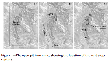
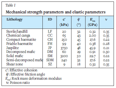
The 2018 pit topography was used to construct the geometric model (Figure 1). The block model of the mine was used to spatially locate the lithologies within the geometric model. Information on the classification of rocks, tests on intact rock, hydrogeological information, geology, and strength properties of the rocks (Table I) were loaded for each lithology present in the model. The finite difference software used for geotechnical modelling was FLAC3D.

 

 

 

 

In both the calibration model and the predictive model, the rock mass behaviour was represented using the elasto-plastic relationship with a failure envelope and ubiquitous joints for all the rock units. The most conservative fabric orientations were selected for each rock type.

 

Calibration of the model

A slope rupture that occurred in 2018 was used to calibrate the strength parameters of the rocks. Figure 1 shows the location of the rupture, and Figure 2 shows the location before and after the rupture.

 

 

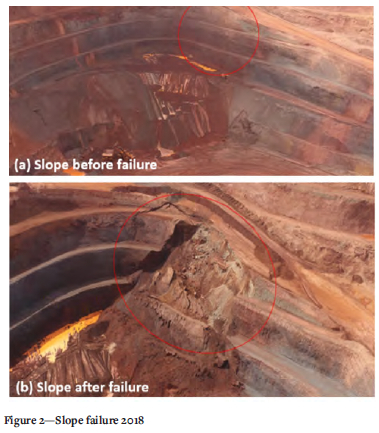
The rupture affected three benches, reaching a maximum height of approximately 45 m. Before and after the occurrence, the slope showed the presence of a large amount of water. The rupture mechanism acting on the slope was interpreted as controlled by the contact between the mafic and iron-beaing rocks, called the shear zone (SZ).

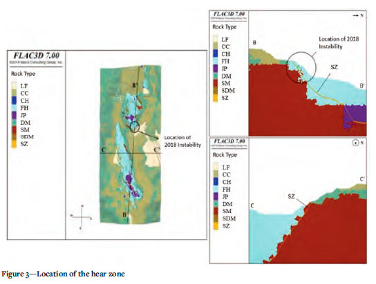
The iron formation consists of friable haematite (FH) and jaspilite (JP) lithotypes (Table I). The mafic formation consists of solid mafic (SM), semidecomposed mafic (SDM), and decomposed mafic (DM) lithotypes. The SZ occurs every where the iron formation overlies the mafic formation. Due to the different densities of these formations, shearing occurs along with relative displacement of the iron formation at the HS/SM, FH, SDM, FH/ DM, JP/SM, JP/SDM, and JP/DM contacts. Figure 3 shows the location of the SZ. In the model, the contact was implemented as a 2 m wide layer.

 

 

Considering a low resistance and an SZ contact plane, the stability of the slope depends on the resistance of the FH lithotype; this lithotype was therefore, the calibrated rock unit.

The calibrated results are presented in terms of numerical velocity contours, which can be compared with the documented instability. The numerical velocity is used as an indicator to interpret the stability conditions in the numerical model. These velocities are given without units because they are mathematical devices used only to represent the convergence of the numerical solution. Wyllie and Mah (2004) and Lorig and Varona (2000) found that velocities below 1e-6 indicate stability in FLAC and FLAC3D; conversely, velocities above 1e-5 indicate instability.

To reproduce the documented instability, it was assumed that the FH lithotype was under saturated conditions (water level near the surface). Under dry conditions, the slopes were stable. The saturation hypothesis was related to the observations documented before and after the rupture. The results in terms of the contour velocities are shown in Figure 4. Good reproduction of this condition was observed, where only the broken slope corresponded to the 2018 instability.

 

 

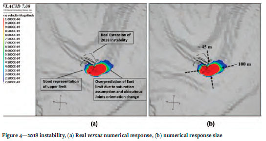
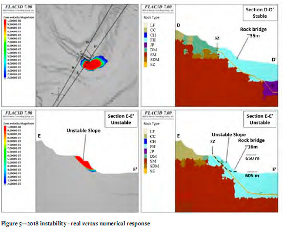
Figure 5 shows that the rupture mechanism is captured well: a planar failure controlled by the SZ contact that occurs when the FH rock bridge breaks. In section E-E', the rock bridge between the SZ contact and the foot of the slope is close to 16 m for a slope 45 m in height. However, in section D-D', where the slope exhibits stable behaviour, the rock bridge between the SZ contact and the foot of the slope is close to 35 m for a 45 m high slope, which presents the slope geometric conditions to avoid instability.

 

 

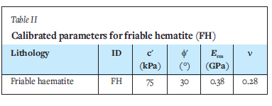
The calibration process modified only the strength properties of the FH lithotype, which mainly participated in the 2018 instability condition. The calibration also defined the strength parameters of the ubiquitous joints used in the model, obeying the more conservative orientations with respect to the orientation of the pit. Table II shows the calibrated properties for the FH lithotype.

 

 

Location of critical stability zones (FoS)

A relevant finding during the calibration process was the importance of the phreatic levels in influencing the behaviour of the slopes. With this in mind, the geometry of the final pit (year 2030) was evaluated considering three alternative hydrogeology scenarios

> Predicted scenario: This scenario uses the inferred phreatic surface for the final pit. This is the most likely predicted case, considering the available information.

> Saturated scenario: This scenario assumes total saturation of the slopes of the final pit. This is the worst possible scenario in terms of groundwater levels.

> Dry scenario: This scenario assumes dry conditions for all slopes of the final pit. This is the best-case scenario in terms of groundwater levels.

The objective of performing three analyses for the final pit was to compare the behaviour of the pit slopes under different groundwater regimes and, therefore, to illustrate the role of groundwater levels in the overall pit stability.

 

Factor of safety (FoS) stability criteria

Figure 6 shows the general behaviour of the pit in terms of the FoS contours. From this graphic, four results can be observed.

 

 

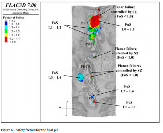
> Unstable areas (FoS < 1.0): These areas are mainly distributed in pit I, pit II, and pit III.

> Areas not in compliance with the acceptability criterion (FoS < 1.3): Although these areas are stable, they do not meet the acceptability criterion. Two cases can be distinguished in this section:

- Areas of marginal stability (1.0 < FoS < 1.1): This area covers a large extension of the east wall of pit I.

- Stable areas that do not meet the acceptability criterion (1.1 < FoS < 1.3): These areas are distributed along the pit.

Unstable areas (FoS <1.o)

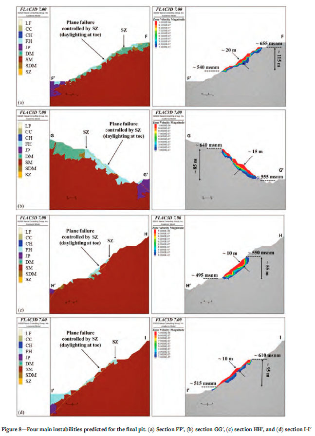
To improve visualization of unstable areas (FoS < 1.0), velocity contours are used as an intermediary between the numerical data and the user to understand the location and extent of the unstable area (Figure 7). The model predicts instabilities on a bench scale (FoS < 1.0; height < 15 m) distributed mainly on the southern slope of pit II and on the eastern slope of pits III and IV. In addition, four large instabilities (FoS < 1.0; height > 50 m) (Figure 8) are predicted. These vary between approximately 50 m and 125 m in height and between 10 m and 20 m in width. They are located on the NE slope of pit I, on the southern slope of pit II, and on the eastern slope of pit III.

 

 

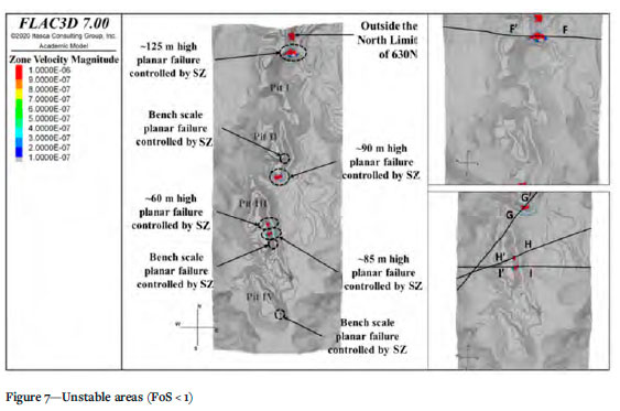
The bench-scale instabilities and the four main instabilities exhibit the same rupture mechanism. In all of them, the SZ shear contact defines a planar rupture geometry. This configuration makes all geometries kinematically admissible for sliding through the SZ shear contact. This geometric configuration makes the prevention of the occurrence of these instabilities ' inevitable', considering the current definition of SZ shear contact.

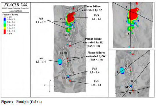
Areas not conforming to the acceptability criteria (1 < FoS < 1.3)

Figure 9 shows the acceptability of the stability of the final pit in terms of FoS contours. Considering that all previously identified instabilities exhibit an FoS < 1.0 (due to their kinematically admissible geometries), the largest extension of the pit exhibits acceptable stability (FoS > 1.3). However, four sectors of the mine raise alarms within the analysis (FoS < 1.3).

 

 

East wall of pit I (section J-J")

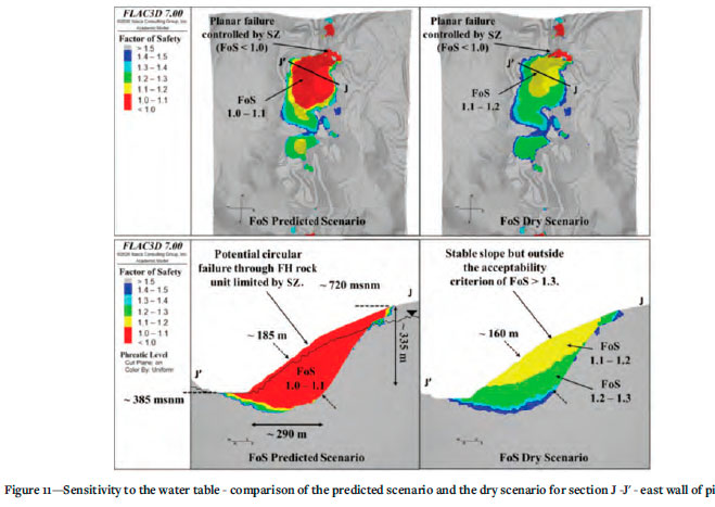
The slope is excavated with an orientation of approximately 300° (D-D') and an IRA of 37° almost exclusively in an FH rock unit. The slope has a convex geometry, promoting lower lateral confinement. The predicted phreatic level is close to the surface at the foot of the slope. Considering the conservative criteria for assigning the different sets of joints, the FH rock unit in this area has ubiquitous joints with an orientation of 72°/282° (dip/ direction of dip). This implies that although the ubiquitous joints have a dip of 72°, they run subparallel to the slope (orientation difference less than 20°). These aspects, applied to an FH rock unit calibrated with 75 kPa of cohesion and friction angle of 30°, result in a slope with an FoS ranging from 1.0 to 1.1. In other words, considering the parameters calibrated for the FH rock unit and the geometric characteristics, this slope shows critical stability. The potential failure mechanism is rupture through the FH rock mass (Figure 10), limited to the east by the SZ and reaching approximiately 335 m. The SZ occurs behind the slope, forming an FH rock bridge of about 290 m. Because the slope is close to the water table, it is important to evaluate the sensitivity of this wall to the position of the water table.

 

 

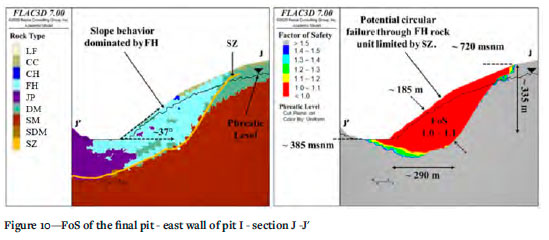
Figure 11 shows the effect of the water table (groundwater position) on the response of the east wall pit I in terms of FoS contours. Compared with that of the predicted scenario, the slope of the dry scenario shows an improvement in FoS contours, with a 0.1 increase in magnitude, going from a critical stability condition to 1.1 < FoS < 1.3. Although the slope continues to exhibit values that do not meet the acceptability criterion, this case shows the sensitivity of the slope to adequate drainage. Based on the results of the FLAC3D model, a change in the IRA angles for the FH rock unit and a change in the east wall design from pit I to the 2030 final pit are recommended.

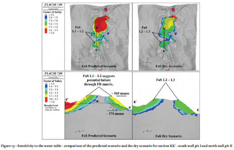
South wall of pit I and north wall of pit II (section K-K^/)

The wall shows FoS contours ranging from 1.1 < FoS < 1.2 (Figure 12), which indicates that the slope is stable but does not meet the acceptability criterion (FoS > 1.3). This wall has two slopes thatdivide pit I and pit II. This wall is built almost entirely in the FH rock unit, with an IRA of approximately 39° for a maximum height of 195 m.

 

 

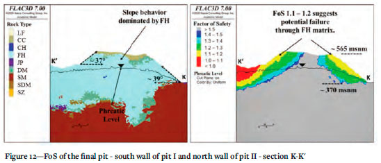
The ubiquitous joints in these domains for the FH in this specific sector have orientations of 59/268 and 57/243, respectively, without affecting the slope performance because the slope orientation is almost E-W. In addition, neither the ubiquitous joints nor the water table affect the magnitude of the FoS contours (Figure 13). This is only a consequence of the resistance envelope of the calibrated FH rock unit. Based on the results of the FLAC3D model, it is also recommended to change the IRAs for the FH rock unit and to change the design of the south wall of pit I and the north wall of pit II to that of the final pit.

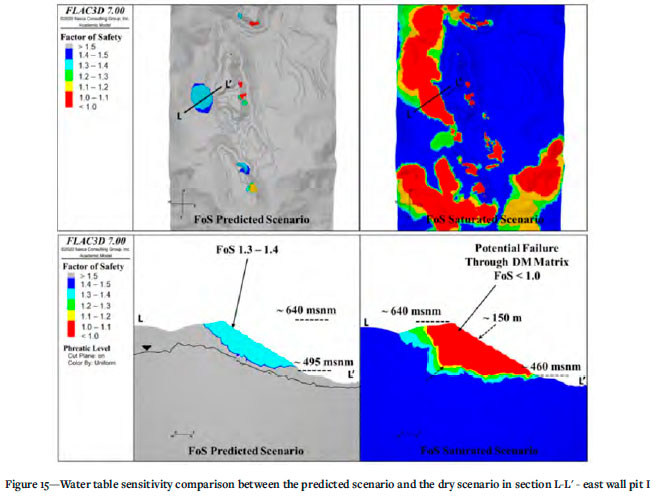
Western wall of pit III (section L-L^r)

The main rock unit in the upper three quarters of the western wall of pit III is DM (Figure 14). This unit (cohesion of 60 kPa, friction angle of 29°) supports a slope of approximately 32° IRA and exhibits FoS contours of 1.3-1.4, where water does not play a significant role in the predicted scenario. Although this slope is in accordance with the acceptability criterion (FoS > 1.3), a sensitivity analysis was performed to evaluate the slope response under the saturated scenario (Figure 15).

 

 

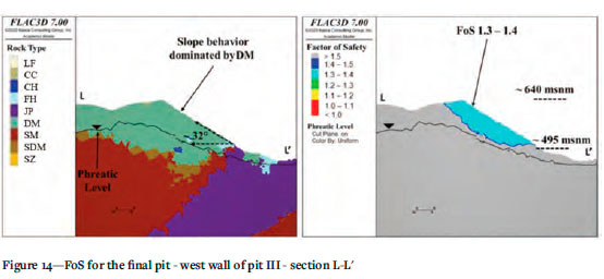
Figure 15 shows the strong sensitivity of the DM, SDM, and FH rock units to the water level, especially in the slope of section L-L', where the wall transitions from an FoS of 1.3-1.4 to an unstable condition (FoS < 1.0) due only to changes in the water table. These results support the recommendation of adequate drainage of the slopes as stability control measures.

East wall of the IV pit (sections M-M and N-N')

The western slope of pit IV has two areas where the SZ forms two planar fault geometries, with rock bridges ranging from approxamately 10 m in the M-M' section to 7 m in the NN' section (Figure 16). The MM' section exhibits critical stability (FoS 1.01.1), with a failure mechanism geometry of up to 90 m in height. For this area, a key factor is the position of the SZ.

 

 

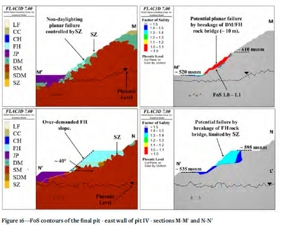
Section NN' shows an FoS of 1.3-1.4. Although the FoS contours meet the acceptability criterion, the integrity of the rock bridge is the key to the stability of the slope.

Discussion of results - 3D stability analysis

The 3D model of the final pit indicates that, to a great extent, the walls meet the acceptability criterion of FoS > 1.3. Considering that several instabilities (FoS < 1.0) up to the bench scale are found (height < 15 m), four main unstable geometries are described (height > 30 m). All of these have the same potential failure mechanism: planar failure geometry controlled by the SZ.

When the FoS contours for the final pit were evaluated, additional information on pit stability was obtained. In the east wall of pit I, the model suggests a stable critical slope (1.0 < FoS < 1.1). This is mainly due to the calibrated parameters for the FH rock unit and the subparallel orientation of the ubiquitous joints. Based on the results of the FLAC3D model, it is necessary to change the IRAs for the FH rock unit and change the design of the east wall from pit I to that of the final pit.

In the south wall of pit I and in the north wall of pit II, the model suggests a stable but not acceptable slope (1.1 < FoS < 1.2). For both slopes, a drop in the water table increases the FoS in increments of 0.1. However, the main factor for the stability behaviour is related to the calibrated strength parameters of the FH rock unit. Based on the results of the FLAC3D model, it is necessary to change the IRA for the FH rock unit and change the design of the south wall of pit I and the north wall of pit II to that of the final pit.

In pit III, the DM rock slope shows 1.3 < FoS < 1.4, which meets the acceptability criterion but shows a strong sensitivity to changes in the water table. In addition to the above slopes, adequate drainage strategies for DM, FH, and SDM slopes are essential.

In pit IV, stability is controlled by the SZ contact shear. The stability depends exclusively on the position of the SZ contact and strength of the rock bridge.

After the areas with critical stability were determined by the 3D stability analysis, the next step was to perform an analysis to determine the PoF of each sector.

 

Probability of failure (PoF)

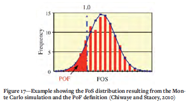
The analysis of the PoF was based on the application of the RSM to the critical sectors of the 2030 final pit. Two steps were performed to obtain the PoF. The first involved the use of a stability model (3DEC) to calculate the FoS for the various combinations of input parameters in the critical sectors, whose responses were fitted to a curve to obtain the total response surface. In the second stage, several realizations were performed with Monte Carlo simulation using the various probability distributions of the parameters. The result of the Monte Carlo simulation was a FoS distribution from which the PoF was calculated (Figure 17).

 

 

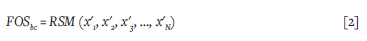
Response surface method (RSM)

The RSM represents the function that defines the distribution of FoS, dependent, for example, on N uncertain variables, such as:

The method assumes that the effect of each xi is independent of the others, where the base case (bc) represents the best estimate value (mean):

The sensitivity of the FoS in relation to the mean values (x_i') is defined by the parameter β as:

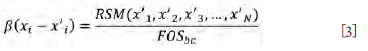
This can be defined in two points on each side of the best estimated value, as shown in Figure 18.

 

 

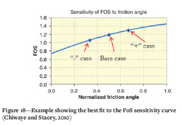
The best-fit curve is obtained for this case, and then any random combination of the input variables can be evaluated by:

Random sampling, such as Monte Carlo simulation, ultimately facilitates the acquisition of the PoF (Figure 17):

In this study, variable input parameters are assumed for the angle of friction and cohesion of the FH and DM units, which are the factors concerning the critical stability of the slopes.

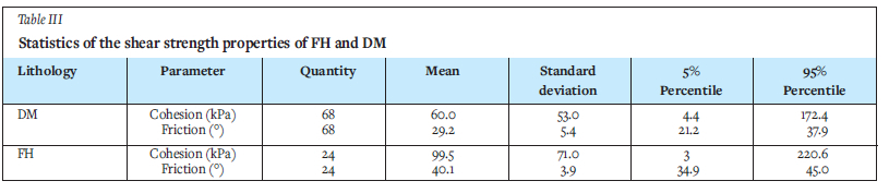
Statistical cases of resistance evaluated

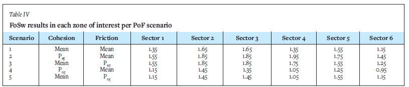
A total of five cases were considered in the PoF analyses: (1) the average properties, (2) cohesion in the 5th percentile (P0₅) and average friction angle, (3) cohesion in the 95th percentile (P₉₅) and average friction angle, (4) average cohesion and friction angle in P0₅, and (5) average cohesion and friction angle in P₉₅. Based on the available laboratory data, the statistics of the resistance properties of FH and DM are shown in Table III.

Critical sectors defined for the probability offailure (PoF) analyses

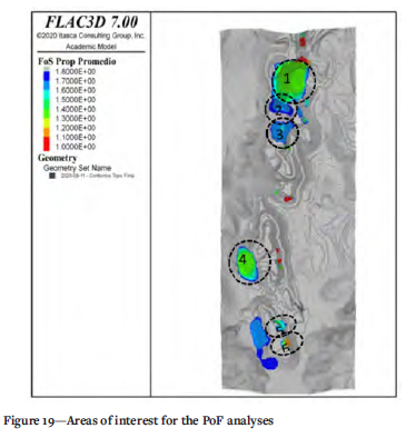
The 3D slope stability model was applied using the average properties to define the zones of interest to calculate the PoF. Figure 19 shows the results of the analysis and indicates the six zones of interest defined for the PoF analyses. The FoS of each zone of interest per PoF scenario is summarized in Table IV.

 

 

Assessment scenarios and PoF

Two scenarios were defined for the PoF calculation. The first scenario (PoF 5-95) assumes that the laboratory data is representative of the population; therefore, the data is used directly as received.

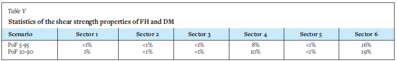
The second scenario (PoF 10-90) assumes that the laboratory data is not completely representative of the population; therefore, it is assumed that P₀₅ of the sample actually corresponds to the 10th percentile of the population, while P₉₅ of the sample is assumed to correspond to the 90th percentile. This scenario is more conservative and helps explain how sensitive the analysis is to variations in some of the assumptions. The RSM was applied to all six sectors of interest. A quadratic fit was used as the best fit for the FoS results, and 10 000 Monte Carlo realizations were generated. The PoF of each sector is shown in Table V.

It is observed that the PoF is typically low, except for two sectors, 4 and 6. The PoF varies from 8% to 10% in sector 4 and from 16% to 19% in sector 6.

It is important to note that the analysis is based on the properties of the materials but the location of the water table is not part of the analysis. As shown in the sensitivity analyses, the location of the water table is a critical stability factor for the pit.

 

Interramp angle (IRA) recommendations

The recommendations for the IRA were developed using a simplified two-dimensional FLAC/Slope v8.0 analysis, considering that the acceptability criterion is FoS > 1.3. The rock units were evaluated for the best and worst cases.

> Best scenario: The analyses were performed for a dry environment, without ubiquitous joints, and the rock mass was represented only by the c, φ of each rock unit.

> Worst case scenario: The analyses were performed for a water table 10 m below the surface for all types of rock, and joints with orientation parallel to the slope plunging in the worst direction.

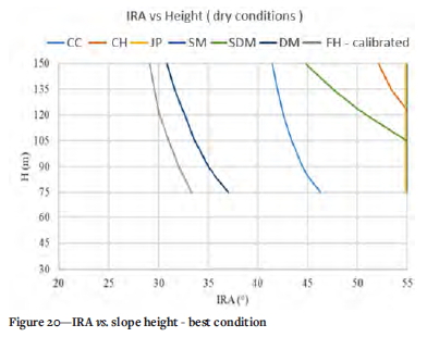
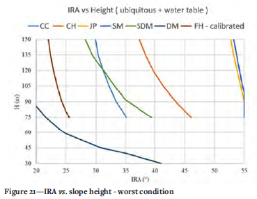
For all rock types (except SM and JP), the friction angle and the cohesion of the ubiquitous joints were considered 50% that of the host rock, while in the SM and JP rock units, they were considered 5% that of the host rock. Figures 20 and 21 show the correlation between the heights of the slopes and IRA for each type of rock. Almost all IRA-height curves exhibit an inverse relationship: the greater the height, the lower the IRA.

 

 

 

 

Factor of safety (FoS) - Probability of failure (PoF)

A total of 240 cases were analysed for each geotechnical unit, and 48 combinations of IRA-slope height (H) for five times the statistical resistance cases evaluated.

For each IRA-H combination, the corresponding PoF was calculated by the RSM methodology, obtaining 48 PoF values. Different PoF isocurves were calculated using the Python matplotlib library (shown in blue in the figures).

As a reference, the FoS curves of the average properties are also plotted in the same figure (shown as discontinuous red lines). Similar to the recommendations of the FoS IRA project, two cases are analysed: dry conditions without ubiquitous joints and conditions with a water table 10 m below the surface and ubiquitous joints.

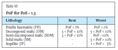
The curves obtained are shown in Figures 22 to 26. Table VI shows the PoF of the slopes according to the lithology for each scenario with a FoS of 1.3.

 

 

Conclusions

The study showed the importance of performing probabilistic analyses to broaden the judgement of the FoS considered acceptable. Two extreme scenarios were evaluated, (1) the best scenario: a dry slope without ubiquitous joints and (2) the worst scenario: a water table at 10 m depth with ubiquitous joints in the most unfavourable direction. The IRA-slope height (H) graphs show the FoS placed between isolines that represent the PoF.

The 3D stability analyses allowed us to divide the final pit into sectors according to the FoS values found. Sectors 1 and 4 presented 1.5 > FoS > 1.3, meeting the acceptability criterion (FoS > 1.3); sectors 2, 3, and 5 were very stable, with FoS > 1.6, while sector 6 presented 1.1 > FoS > 1.3 stable areas that did not meet the acceptability criterion.

The probabilistic analyses for all evaluated sectors considered two statistical scenarios. In the first scenario (5 < PoF < 95), it was assumed that the laboratory data is representative of the population. In the second scenario (10 < PoF < 90), it was assumed that the laboratory data is not completely representative of the population, and the scenario was more conservative. The probabilistic analysis used 10 000 Monte Carlo realizations. The results showed that for sectors 1, 2, 3, and 5, the PoF is < 1%, while for sectors 4 and 6, the PoF is between 8% < PoF < 10% and 16% < PoF < 19%, respectively.

The high PoF of sector 6 verifies the results of the stability analyses previously performed, which is not the case with sector 4, where the criterion of acceptability of the stability of the sector is met (FoS > 1.3) but the PoF can be considered high (8% < PoF < 10%) compared to those of the other sectors considered stable.

In conclusion, the results show that probabilistic evaluation is an important tool for establishing alert mechanisms in slopes that can be termed stable. In addition, it broadens the view of those responsible for mine planning when deciding the slope of the IRA, especially when the purpose of the mine is to remove as much material as possible under stability criteria that ensure the safety of the slopes, consequently increasing the reliability of operations and improving the mine safety system.

 

Data availability statement

All data, models, and code generated or used during the study appear in the submitted article.

 

Acknowledgements

We thank Vale SA for providing the data and the Vale Institute of Technology for guidance and support in this work.

 

References

Chiwaye, H.T. and Stacey T.R. 2010. A comparison of limit equilibrium and numerical modelling approaches to risk analysis for open pit mining. Journal of the Southern African Institute of Mining and Metallurgy, vol. 110. pp. 571-580.         [ Links ]

Chowdhury, R.N. and Xu, D.W. 1995. Geotechnical system reliability of slopes. Reliability Engineering & System Safety, vol. 47, no. 3. pp. 141-151.         [ Links ]

Contreras, L.F. 2015. An economic risk evaluation approach for pit slope optimization. Journal of the Southern African Institute of Mining and Metallurgy, vol. 115, no. 7. pp. 607-622.         [ Links ]

El-Ramly, H., Morgenstern, N.R., and Cruden, D.M. 2002. Probabilistic slope stability analysis for practice. Canadian Geotechnical Journal, vol. 39, no. 3. pp. 665-683.         [ Links ]

Griffiths, D.V. and Fenton, G.A. 2004. Probabilistic slope stability analysis by finite elements. Journal of geotechnical and geoenvironmental engineering, vol. 130, no. 5. pp. 507-518.         [ Links ]

Hicks, M.A., Nuttall, J.D. and Chen, J. 2014. Influence of heterogeneity on 3D slope reliability and failure consequence. Computers and Geotechnics, vol. 61. pp.198-208.         [ Links ]

Huang, J., Lyamin, A.V., Griffiths, D.V., Krabbenhoft, K., and Sloan, S.W. 2013. Quantitative risk assessment of landslide by limit analysis and random fields. Computers and Geotechnics, vol. 53. pp. 60-67.         [ Links ]

Ji, J. and Low, B.K. 2012. Stratified response surfaces for system probabilistic evaluation of slopes. Journal of Geotechnical and Geoenvironmental Engineering, vol. 138, no. 11. pp. 1398-1406.         [ Links ]

Jiang, S.H., Li, D.Q., Zhang, L.M., and Zhou, C.B. 2014. Slope reliability analysis considering spatially variable shear strength parameters using a non-intrusive stochastic finite element method. Engineering Geology, vol. 168. pp. 120-128.         [ Links ]

Johari, A. and Gholampour, A. 2018. A practical approach for reliability analysis of unsaturated slope by conditional random finite element method. Computers and Geotechnics, vol. 102. pp. 79-91.         [ Links ]

Kasama, K. and Whittle, A.J. 2016. Effect of spatial variability on the slope stability using random field numerical limit analyses. Georisk: Assessment and Management of Risk for Engineered Systems and Geohazards, vol. 10, no. 1. pp. 42-54.         [ Links ]

Kasama, K., Fürükawa, Z., and Hu, L. 2021. Practical reliability analysis for earthquake-induced 3D landslide using stochastic response surface method. Computers and Geotechnics, vol. 137. p. 104303.         [ Links ]

Le, T. 2014. Reliability of heterogeneous slopes with cross-correlated shear strength parameters. Georisk: Assessment and Management of Risk for Engineered Systems and Geohazards, vol. 8, no. 4. pp. 250-257.         [ Links ]

Li, D.Q., Qi, X.H., Phoon, K.K., Zhang, L.M., and Zhou, C.B. 2014. Effect of spatially variable shear strength parameters with linearly increasing mean trend on reliability of infinite slopes. Structural safety, vol. 49. pp. 45-55.         [ Links ]

Li, D.Q., Wu, S.B., Zhou, C.B., and Phoon, K.K. 2012. Performance of translation approach for modeling correlated non-normal variables. Structural safety, vol. 39. pp. 52-61.         [ Links ]

Li, D.Q., Xiao, T., Cao, Z., Zhou, C., and Zhang, L. 2016. Enhancement of random finite element method in reliability analysis and risk assessment of soil slopes using Subset Simulation. Landslides, vol. 13, no. 2. pp. 293-303.         [ Links ]

Li, D.Q., Zheng, D., Cao, Z.J., Tang, X.S., and Phoon, K.K. 2016. Response surface methods for slope reliability analysis: review and comparison. Engineering Geology, vol. 203. pp. 3-14.         [ Links ]

Li, L. and Chu, X. 2015. Multiple response surfaces for slope reliability analysis. International Journal for Numerical and Analytical Methods in Geomechanics, vol. 39, no. 2. pp. 175-192.         [ Links ]

Liu, Y., Zhang, W., Zhang, L., Zhu, Z., Hu, J., and Wei, H. 2018. Probabilistic stability analyses of undrained slopes by 3D random fields and finite element methods. Geoscience Frontiers, vol. 9, no. 6. pp. 1657-1664.         [ Links ]

Lorig, L. and Varona, P. 2000. Practical slope-stability analysis using finite-difference codes. Slope stability in surface mining. pp. 115-124.         [ Links ]

Malkawi, A., Hassan, W., and Abdulla, F. 2000. Uncertainty and reliability analysis applied to slope stability. Structural safety, vol. 22, no. 2. pp. 161-187.         [ Links ]

Mellah, R., Auvinet, G., and Masrouri, F. 2000. Stochastic finite element method applied to non-linear analysis of embankments. Probabilistic Engineering Mechanics, vol. 15, no. 3. pp. 251-259.         [ Links ]

Phoon, K. and Kulhawy, F.H. 1999. Characterization of geotechnical variability. Canadian geotechnical journal, vol. 36, no. 4. pp. 612-624.         [ Links ]

Read, J. and Stacey, P. 2009. Guidelines for Open Pit Slope Design, CSIRO Publishing, Collingwood, Victoria, 496 pp.         [ Links ]

Soares, R.C., Mohamed, A., Venturini, W.S., and Lemaire, M. 2002. Reliability analysis of non-linear reinforced concrete frames using the response surface method. Reliability Engineering & System Safety, vol. 75, no. 1. pp. 1-16.         [ Links ]

Terbrugge, P.J., Wesseloo, J., Venter, J., and Steffen, O.K.H. 2006. A risk consequence approach to open pit slope design, Journal of the Southern African Institute of Mining and Metallurgy, vol. 106, no. 7. pp. 503-511.         [ Links ]

Wyllie, DC. and Mah, C. 2004. Rock slope engineering: Civil and mining (4th ed.). London, CRC Press, London,. pp. 231-232.         [ Links ]

Wong, F.S. 1985. Slope reliability and response surface method. Journal of geotechnical Engineering, vol. 111, no. 1. pp. 32-53.         [ Links ]

Xiao, T., Li, D.Q., Cao, Z.J., Au, S.K., and Phoon, K.K. 2016. Three-dimensional slope reliability and risk assessment using auxiliary random finite element method. Computers and Geotechnics, vol. 79. pp. 146-158.         [ Links ]

Xu, B. and Low, B.K. 2006. Probabilistic stability analyses of embankments based on finite-element method. Journal of Geotechnical and Geoenvironmental Engineering, vol. 132, no. 11. pp. 1444-1454.         [ Links ]

Zhang, J., Zhang, L.M., and Tang, W.H. 2011. New methods for system reliability analysis of soil slopes. Canadian Geotechnical Journal, vol. 48, no. 7. pp.1138-1148        [ Links ]

 

 

Correspondence:
J.M. Girao Sotomayor
Email: juan.sotomayor@itv.org

Received: 14 Oct. 2021
Revised: 8 Mar. 2022
Accepted: 16 Mar. 2022
Published: July 2022