PROFESSIONAL TECHNICAL AND SCIENTIFIC PAPERS

 

Investigation of the mixing characteristics of industrial flotation columns using computational fluid dynamics

 

 

I. Mwandawande^I; S.M. Bradshaw^I; M. Karimi^II; G. Akdogan^I

^IUniversity of Stellenbosch, Process Engineering, South Africa
^IIDepartment of Chemistry and Chemical Engineering, Chalmers University of Technology, Sweden

Correspondence

 

 

---

SYNOPSIS

The mixing characteristics of industrial flotation columns were investigated using computational fluid dynamics (CFD). Particular emphasis was placed on the clarification of the relationship between the liquid and solids mixing parameters such as the mean residence time and axial dispersion coefficients. The effects of particle size and bubble size on liquid dispersion in the column were also studied. An Eulerian-Eulerian method was applied to simulate the multiphase flow, while additional scalar transport equations were introduced to predict the liquid residence time distribution (RTD) and particle age distribution inside the column. The results obtained show that particle residence time decreases with increasing particle size. The residence time of the coarser particles (112.5 pm) was found to be at least 60% of the liquid residence time, while the finer particles (19 pm) had a residence time similar to the liquid. The results also show that an increase in the particle size of the solids results in a decrease in the liquid vessel dispersion number, while a decrease in the bubble size increases liquid axial mixing. Finally, the simulated axial velocity profiles confirm the similarity between the liquid and solids axial dispersion coefficients in column flotation.

Keywords: mixing characteristics, flotation column, computational fluid dynamics, residence time distribution.

---

 

 

Introduction

Column flotation is an established mineral concentration technology used in the mineral processing and coal beneficiation industries. The concentration process takes place through the collection of valuable hydrophobic mineral particles by a rising swarm of air bubbles in countercurrent flow against a feed slurry in the collection zone of the column. The bubbles then transport the mineral particles to the top of the column into the froth zone (or cleaning zone) where the particles are eventually recovered in the overflow.

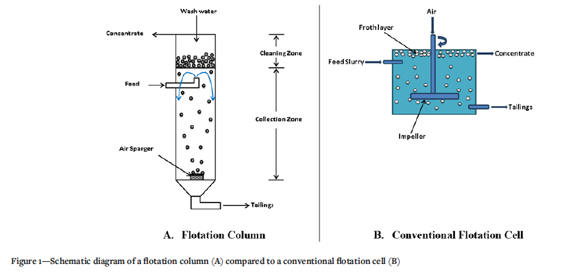
Flotation columns differ from conventional flotation cells in a number of ways. For example, in column flotation the bubbles are generated using spargers located at the bottom of the column, while impellers are used in conventional cells for this purpose. In addition, wash water is added into the froth zone at the top of the flotation column to wash down any unwanted particles entrained from the collection zone. This feature is not present in conventional cells. The froth layer formed at the top part of the flotation column is also deeper compared to conventional cells. This is because of the stabilizing effects from the wash water which is added into the froth zone. The main differences between columns and conventional cells are illustrated in Figure 1.

Flotation columns are known for their improved metallurgical performance compared to conventional flotation cells. In particular, the addition of wash water enables flotation columns to produce higher concentrate grades compared to conventional cells, which usually produce lower grades due to particle entrainment. In addition, the required concentrate grades are achieved in a single-stage process in flotation columns, whereas conventional cells require several stages to obtain a suitable grade (Finch and Dobby, 1990). However, increased mixing in the column can adversely affect its grade and recovery performance. It has been observed that mineral recovery decreases as the mixing conditions increase from plug flow towards perfectly mixed flow in the column (Finch and Dobby, 1990). As a result, the design and optimization of flotation columns require detailed knowledge of the effects of various geometrical and operational parameters on the mixing characteristics of the column.

The mixing characteristics of flotation columns have been studied by several researchers (Dobby and Finch, 1985; Mills, Yionatos, and O'Connor, 1992; Yianatos and Bergh, 1992; Yianatos et al., 2005; Xu and Finch, 1992). However, there are still uncertainties, particularly with regard to solids mixing characteristics in the column. The earlier studies by Dobby and Finch (1985) and Yianatos and Bergh (1992) suggested that the solids and liquid axial dispersion coefficients were equal. On the other hand, several authors have questioned the equivalence of the solids and liquid dispersion, citing various reasons (Ityokumbul, Kosaric, and Bulani, 1988; Mills and O'Connor, 1990; Goodall and O'Connor, 1991; Ityokumbul, 1992). Ityokumbul, Kosaric, and Bulani (1988) argued that the observed equivalence of the solids and liquid axial dispersion coefficients in the work of Dobby and Finch (1985) could have been based on wrong experimental data. In particular, they suggested the possible presence of dead volumes in the column that was used in the experiments and the use of wrong boundary conditions in the subsequent calculations as the main problems. On the other hand, Mills and O'Connor (1990) observed that the feed percentage solids used in the work of Dobby and Finch was too low to highlight differences between the liquid and solids axial dispersion coefficients. They then demonstrated, using their own experimetal work, that the solids axial dispersion coefficient did not equal the liquid one. Other notable arguments against the equivalence of liquid and solids dispersion coefficients are presented by Ityokumbul (1992), who went further to question the applicability of the axial dispersion model for describing the behaviour of solid particles by previous researchers.

Some researchers have also investigated the effect of solids on the liquid dispersion in the column (Finch and Dobby, 1991). It has been reported that the liquid dispersion decreases as the percentage of solids in the feed increases, possibly due to viscous effects. However, the effect of particle size on the liquid dispersion has not yet been studied.

The studies described above were entirely based on experimental methods in which the solids and liquid velocity fields inside the column were not examined. Computational fluid dynamics (CFD) is an alternative modelling tool which is based on the flow physics of the process. CFD methodology can therefore be used to study the mixing characteristics of flotation columns, with the additional advantage of basing the interpretation of the results on the detailed velocity fields derived from numerical simulations.

Over the last two decades, CFD has emerged as a powerful tool for modelling the flotation separation process. The focus has been mostly on conventional flotation cells, where the hydrodynamics are coupled with flotation sub-processes such as bubble-particle collision, attachment, and detachment (Koh, Manickam, and Schwarz, 2000; Koh and Schwarz, 2009; Liu and Schwarz, 2009; Koh and Schwarz, 2006). Nonetheless, only a limited amount of CFD literature is available for column flotation, as this process is typically modelled through extensive large-scale experimentations.

One of the earliest numerical works is that by Deng, Mehta, and Warren (1996), who applied two-phase numerical simulations to study the two-dimensional flow of flotation columns. Using the axis-symmetric assumption, they reported a liquid circulation pattern in which the axial liquid velocity was upward in the centre and downward near the walls of the column. The liquid circulation established in the column was subsequently cited as one of the main reasons for mixing in column flotation. In addition, the effect of superficial gas velocity on the extent of mixing in the column was investigated. An increase in superficial gas velocity was reported to cause more liquid circulation, which would result in increased mixing in the column. However, the actual mixing was not simulated in terms of residence time distributions (RTDs) and the flow was assumed to be laminar, which eliminates the significant effect of turbulent eddies on the mixing.

Subsequent studies were conducted by Xia, Peng, and Wolfe (2006) who used a Lagrangian two-dimensional CFD model to simulate the alleviation of liquid back-mixing by baffles and packing in a flotation column. Their study revealed that the liquid back-mixing in an open flotation column could be alleviated by using baffles and packing. In addition, the effects of different operating conditions such as uneven aeration, superficial gas velocity, and bubble size on liquid flow patterns in the column were also studied. In this regard, a decrease in bubble size was reported to cause an increase in the upward axial liquid velocity, resulting in a possible increase in liquid back-mixing in the column. However, liquid RTD simulations in order to quantify the effect of the various geometrical and operational conditions on the actual mixing parameters in the column were not conducted.

Contrary to Xia, Peng, and Wolfe, Chakraborty, Guha, and Banerjee (2009) applied an Eulerian-Eulerian approach with k-ε turbulence model to investigate the influence of geometrical and operational parameters on the hydrodynamics of a tapered column. Their study found that increasing the air flow rate resulted in an increase in gas holdup and complexity in the bubble plume structure. In addition, increasing the column height-to-diameter ratio was also observed to bring about a complex flow pattern with multiple staggered vortices in the column. A low height-to-diameter ratio was therefore recommended as one of the required conditions for obtaining good separation in a column flotation cell.

Simulations on the scale of bubbles and particles are also reported in literature. For example, Nadeem, Ahmed, and Chughta (2006) and Koh and Schwarz (2009) presented CFD-based models to predict the flotation sub-processes in column flotation and Jameson cells. As regards columns they applied a Eulerian-Lagrangian method to predict the bubble-particle collision rate in a small rectangular shape domain with a stationary bubble positioned at the centre. For Jameson cells, however, they applied a Eulerian-Eulerian framework to account for the rate of collision, attachment, and detachment of bubbles and particles.

Rehman et al. (2011) investigated the effect of various perforated baffle designs on air holdup and mixing in a flotation/ bubble column using CFD. The Eulerian-Eulerian multiphase model was utilized in the simulations together with the standard k-ε turbulence model. To reduce the computational cost, simulations were performed only for one quarter of the column geometry using a rotational periodic boundary condition to periodically repeat the results for the entire column. The trays (baffles) were observed to significantly increase the overall air holdup compared to the column without baffles.

Most of the CFD models in the literature have assumed a constant bubble diameter. However; Sarhan, Naser, and Brooks (2016) incorporated a population balance equation (PBE) into a two-fluid model to predict the number density of different bubble size classes in a flotation column. This study found that the presence of solids reduced the gas holdup in the flotation cell (column). The authors also reported that the size of gas bubbles decreased with increasing superficial gas velocity, causing the gas holdup to increase. Their results further showed that the Sauter mean bubble diameter decreased with increasing solids concentration.

More recently, Mwandawande et al. (2019) investigated the application of CFD for predicting not only the average gas holdup, but also the axial gas holdup variation in flotation columns. They applied a Eulerian-Eulerian multiphase model and the realizable k-ε turbulence formulation to simulate a cylindrical pilot column that was used in the work of Gomez et al. (1991) and Gomez et al. (1995) on axial gas holdup distribution. Their work further investigated axial bubble velocity profiles to establish possible relationship with the axial gas holdup profile along the column height. The predicted average gas holdup values were found to be in good agreement with experimental data. On the other hand, the axial gas holdup prediction was generally good for the middle and top parts of the column, while the gas holdup was over-predicted for the bottom part of the column.

In another recent study, Mwandawande et al. (2019b) investigated the maximum superficial gas velocity for transition from bubbly flow to churn-turbulent flow in flotation columns using CFD. Their research employed radial gas holdup profiles and gas holdup versus time graphs to identify the loss of bubbly flow in a pilot-scale column flotation cell. The bubbly flow regime was found to be characterized by saddle-shaped profiles with three distinct peaks, or saddle-shaped profiles with two near-wall peaks and a central minimum point, or flat profiles with intermediate features between saddle and parabolic gas holdup profiles. On the other hand, parabolic profiles were observed beyond bubbly flow conditions. For the gas holdup versus time graphs, churn-turbulent flow conditions were characterized by wide variations in the gas holdup versus time graph while gas holdup is almost constant under bubbly flow conditions.

From the literature reviewed above, it is clear that CFD modelling has emerged as a vital tool which has been successfully applied to investigate various aspects of the column flotation process. However, there still exists a clear gap in the current literature regarding the mixing characteristics of industrial flotation columns. For example Deng, Mehta, and Warren (1996) presumed that liquid recirculation is the main reason for mixing while neglecting the effects of turbulence in the column. This assumption oversimplifies the actual physics causing the mixing phenomenon. Furthermore, the actual mixing was not simulated in terms of RTDs. The subsequent work of Xia, Peng, and Wolfe (2006) also did not account for the RTD of the liquid within the column.

The previous CFD models encountered in the literature are all limited to only two-phase systems (gas-liquid) in which mineral particles are not considered. The mixing characteristics of solids in column flotation have therefore not been studied in the previous CFD models. It is also important to note that the previous CFD research pertaining to mixing in column flotation was conducted on laboratory-scale columns - simulations concerning industrial columns have not yet been reported. The main contribution of the study presented in this paper is therefore to investigate the mixing characteristics of industrial flotation columns using CFD.

The mixing characteristics of the flotation column are studied with particular focus on solids mixing and the effects of particle and bubble sizes on the liquid axial dispersion. In this regard, CFD modelling was applied to simulate the 0.91 m diameter cylindrical column from the work of Yianatos and Bergh (1992). The data from these authors is therefore used to validate the present modelling approach. The work presented in this paper involves numerical simulations of RTDs of both the liquid and solid phases in the industrial column. The simulated RTDs are then used to determine the mixing parameters, i.e., the mean residence time and the vessel dispersion number. Both the mean residence time and the vessel dispersion number are useful parameters in the design and scale-up equations for column flotation. In addition, the simulated axial velocity profiles of the solids and liquid phases are compared in order to clarify the relationship between the solids and liquid dispersion characteristics.

 

Theory

The one-dimensional (axial) plug flow dispersion model is applicable to describe the axial mixing process in the collection zone of the flotation column (Finch and Dobby, 1990). In this case, the degree of mixing is quantified by the axial dispersion coefficient D (units of length²/time) or the dimensionless vessel dispersion number (N_d )The higher the vessel dispersion number, the higher the degree of mixing. The vessel dispersion number is given by:

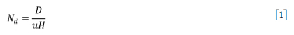
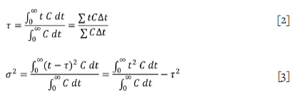
where u is either the liquid interstitial velocity or the particle velocity and H is the height of the collection zone. The axial dispersion coefficient (D) or the vessel dispersion number (N_d ) can be calculated from RTD data using two parameters: the mean residence time (τ) and the variance (σ²). The variance is a measure of the spread of the RTD curve, which represents the degree of mixing within the vessel. It has units of (time)².

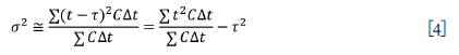
From the RTD data, the mean residence time (τ) and variance (σ²) are calculated from the following equations:

For a set of discrete data-points, the variance is expressed as:

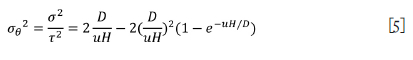
The vessel dispersion number ( is then calculated from the mean residence time and the variance from the following equation for closed vessel boundary conditions (Levenspiel, 1972):

 

CFD methodology

Multiphase model

The CFD simulations in this study are conducted using the Ansys Fluent 14.5 software package in which the finite volume method is applied to convert a system of partial differential equations into algebraic equations that can be solved numerically. In the finite volume method, the computational domain is first discretized into a finite number of control volumes (cells) where general transport equations for mass, momentum, and energy are solved numerically to obtain the solution field. The Eulerian-Eulerian (E-E) multiphase model, in which the continuous (primary) phase and the dispersed (secondary) phases are modelled in an Eulerian frame of reference as interpenetrating continua, is used in this research to simulate the three-phase (gas-liquid-solids) flow prevailing in industrial flotation columns.

In the E-E model, the conservation equations for mass and momentum are solved separately for all three phases in the flow, while interactions between the phases are accounted for with the interphase force exchange term (i.e., R ) as well as other forces such as the lift force and virtual mass force included in the momentum equations (Equation [7]). On the other hand, the volume fraction of the secondary phases is calculated from the continuity (or mass conservation) equation by dividing all the terms with the volume-averaged density of the respective phase in the solution domain. The volume fraction of the primary phase is then calculated based on the condition that all the volume fractions sum to unity.

In the present study, the three-phase flow in the industrial column is modelled considering water as the continuous (or primary) phase while air bubbles and solid particles are treated as dispersed (or secondary phases). In terms of momentum exchange forces between the phases, the drag force between the continuous phase and the dispersed phases is the only significant interfacial force in the multiphase flow. Minor forces such as lift and virtual mass are therefore not included in the model.

For the solid phase momentum equations additional terms derived from the kinetic theory of granular flows are also included to account for the behaviour of solid particles in the multiphase flow. These terms account for particle-particle collisions and the kinetic energy contained in the random motion of the particles. The kinetic theory of granular flows is based on the assumption that the behaviour of solid particles in multiphase flow is similar to the motion of molecules in a gas. Classical results from the kinetic theory of gases are therefore employed to formulate transport equations for the solid phase in the granular flow.

Governing equations

The general forms of mass and momentum conservation equations for each phase are given in Equations [6] and [7], where represents the ^th phase:

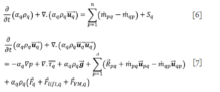
In these equations, á_q is the volume fraction of phase is the velocity, p_q is the density, m_pq represents mass transfer from phase p to phase q, and m_pq is the mass transfer from phase q to phase p. However, mass transfer between phases was not considered in the present study. On the other hand, the source term S_q was only specified for the gas phase to represent the bubbles entering at the bottom of the column and leaving at the top.

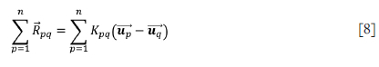
The term in the momentum equation (Equation [7]) is the interaction force between the phases, which in Ansys Fluent represents the drag fo rce, while the other forces such as the external body force , the lift force , and the virtual mass force are added separately if required in the simulations, as shown in Equation [7]. In the present study, the external body force is included in the momentum equation for the gas phase as a momentum source term associated with the mass source terms representing the entry of the air bubbles at the bottom of the column. However, the lift force and virtual mass force are in most cases insignificant compared to the drag force. The present work therefore considers only the drag force in the simulations and the lift and virtual mass forces are left out. The drag force is given by:

where K_pq (=K) is the momentum exchange coefficient, which is described later. The gravity force is included as and p is the pressure which is shared by all phases while T_q is the stress tensor for phase q given by:

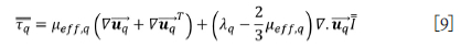
where is the effective viscosity, which is the sum of the molecular viscosity (μΚ) and the turbulent viscosity (μ ), is the bulk viscosity of phase q, and I is the identity matrix. The molecular viscosity is a single-phase material property, while the turbulent viscosity depends on the characteristics of the flow. In order to determine the turbulent viscosity a turbulence model is employed in the simulations as described in the following section.

For the solid phase the governing equations are modified with derivations from the kinetic theory of granular flows to model fluid-solid multiphase systems as mentioned earlier. In Ansys Fluent this is achieved by activating the Eulerian-granular model. In this case, additional terms are incorporated in the solid phase momentum equations to account for the effects of particle collisions based on analogies between the random particle motions arising from interparticle collisions and the thermal motion of gases. The subsequent equations and detailed derivations are available in the Ansys Fluent Theory Guide (Ansys Inc, 2013) and will not be presented here for brevity purposes.

Turbulence model

In the present study, the turbulent viscosity in the continuous phase (water) was calculated using the realizable k-e turbulence model as follows:

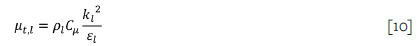
where the turbulent kinetic energy k and the turbulent dissipation rate ε are computed from their respective transport equations while the variable C_p is calculated as described by Shih (1997). The present study utilizes the dispersed k-e turbulence model option which is available in Ansys Fluent for simulating multiphase systems where there is clearly one primary continuous phase with dispersed dilute secondary phases. In this case, turbulence in the continuous or primary phase is considered to be the dominant process in the flow. Transport equations for turbulence (k and e) are therefore solved for the continuous phase only, while turbulence quantities for the secondary phases are calculated using Tchen theory, in which the particle or bubble fluctuations are assumed to be driven by the surrounding continuous phase. The dispersed phase properties are thus obtained from continuous phase properties using algebraic relationships as elaborated in the Ansys Fluent Theory Guide (Ansys Inc, 2013). In addition, the dispersed k-e turbulence model accounts for turbulence modification by the secondary phases through additional terms that incorporate interphase turbulent momentum transfer. The turbulence quantities near the column wall were obtained using algebraic correlations (standard wall functions) to avoid the computational effort associated with alternative methods such as mesh refinement of the way region.

Interphase momentum transfer and drag coefficient

Gas-liquid drag

In order to solve the governing equations for the E-E model, closure models are required for the interphase force R_pq representing the drag between the primary phase and the secondary phase. The exchange coefficient K_pq for bubbly flows can be written as:

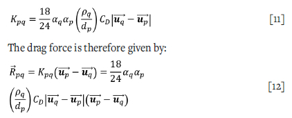
where C_D is the is the drag coefficient between the liquid phase (phase q) and the air bubbles (phase p), d_p is the bubble diameter, and is the slip velocity. Four different average bubble sizes, including 0.8, 1, 1.5, and 2 mm, were used in the simulations. However, validation of the model results against experimental data was done using the simulations conducted with 0.8 mm bubble size only since this is the typical size of bubbles in industrial flotation columns.

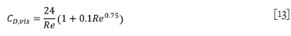
There are a number of empirical correlations that can be used to calculate the drag coefficient (C_D). In the present study, the drag coefficient is calculated using the universal drag laws (Kolev, 2005). The universal drag coefficient is in this case defined in different ways, depending on whether the prevailing regime is in the viscous regime category, the distorted bubble regime, or the strongly deformed capped bubbles regime. At the moderate superficial gas velocities simulated in the present study, the viscous regime conditions apply and the drag coefficient is calculated from the following equation:

The drag coefficient is therefore expressed as a function of the bubble Reynolds number (Re) which is defined as:

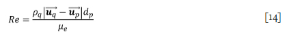
where μ_e is the effective viscosity of the primary phase (i.e. water) modified to account for the presence of the secondary phase (air bubbles in this case).

Liquid-solid drag

The drag force between the liquid and the solid particles is calculated using the Wen and Yu (1966) drag model. In this case, the fluid-solid exchange coefficient is given by:

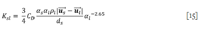
The drag coefficient is then calculated as:

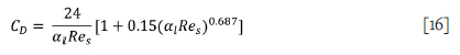
where d_s is the diameter of the solid particles and Re_s is the relative Reynolds number given by

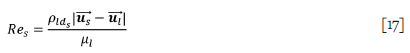
The Wen and Yu model is suitable for dilute systems similar to the conditions simulated in the present study.

Model geometry, mesh, and boundary conditions Computational domain and mesh

Flotation columns are divisible into two distinct zones (refer to Figure 1) - the collection zone and the cleaning zone (or froth zone). It is therefore important to define the computational domain being simulated in the flotation column CFD model. Due to the differences in flow patterns and turbulence characteristics between the collection zone and the froth zone, it still remains a challenge to formulate CFD simulations that combine the two zones. The present research therefore focuses on the collection zone only. Since only the collection zone is modelled, the model geometry is simply a cylindrical vessel of height equal to the collection zone height and radial dimensions similar to the simulated industrial column.

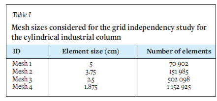
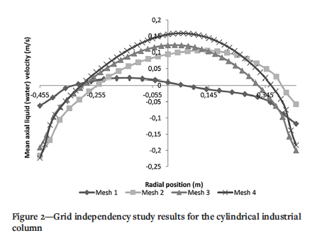
A three-dimensional mesh comprising mainly hexahedral elements is generated over the cylindrical column geometry and used in the subsequent CFD simulations. As a preliminary stage for the simulations, a grid independency study is performed in which different flow variables are compared at different mesh sizes in order to check the dependency of the solution on the grid size. The details of the mesh sizes used in the grid independency study are reported Table I. The results are presented in Figure 2, where the water axial velocity profiles are compared as a function of cell numbers. As seen, the choice of element sizes initially yields unrealistic velocity profiles, while after mesh 3 (2.5 cm cell size with 502 098 cells) the velocity profiles show only small variations with regard to the cell size. However, the computational effort required to perform the simulations beyond mesh 3 becomes unreasonably high. The mesh comprising 2.5 cm mesh with 502 098 elements (or cells) is therefore selected for the subsequent simulations in the column, albeit as only a reasonable trade-off between accuracy and computational effort required for the simulations.

 

 

 

 

Modelling of the spargers

The sparging of gas into the column was modelled using mass source terms introduced in the gas-phase continuity equations for the computational cells at the bottom of the column. Corresponding momentum source terms are also included in the gas-phase momentum equations. The gas phase is assumed to enter the column as air bubbles. In industrial flotation columns the spargers distribute bubbles uniformly over the entire column cross-section (Harach, Wates, and Redfearn, 1990). The air bubbles were therefore introduced over the entire column cross-section in the CFD model without including the physical spargers in the model geometry. The mass source terms and their associated momentum in the upward direction are calculated from the superficial gas velocities as follows:

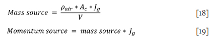
where p_air is the density of air (1.225 kg/m³), A_c is the column cross-sectional area (m²), J_g is the superficial gas (air) velocity (m/s), and V is the volume of the cell zone where the source terms are applied. Corresponding sink terms are also applied at the top of the column to simulate the exit of the air bubbles from the collection zone.

Boundary conditions

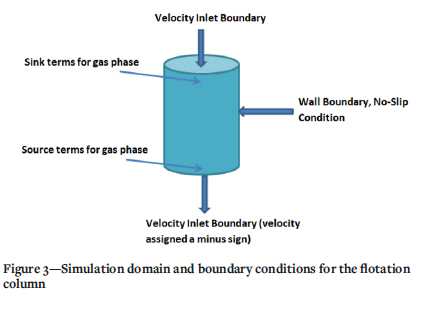
The top of the collection zone of the column was modelled as a velocity inlet boundary for the liquid and solid phases. Inlet velocity magnitudes normal to the boundary are therefore prescribed together with turbulence parameters to enforce a Dirichlet-type boundary condition at the face. For the liquid phase, the inlet velocity was specified as equal to superficial liquid velocity (J,). Since the computational domain being considered is the collection zone of the column, the superficial liquid velocity must include the feed rate plus the bias water resulting from wash water addition. The superficial liquid velocity is therefore equal to the superficial tailing rate (J₍). Turbulence parameters at the inlet boundary were prescribed by setting the turbulence intensity equal to 5%. This value is recommended for fully developed turbulent flow upstream of the boundary face (Ansys Inc, 2013). Fully developed flow conditions were therefore assumed at the inlet boundary.

The solid particles are assumed to be transported into the column at the same velocity as the surrounding liquid phase. Similar superficial velocity values were therefore used to describe the solids boundary conditions. In addition, the phase volume fractions of the solids in the liquid were specified at the inlet boundaries.

The bottom part of the column was also modelled as a velocity inlet boundary for both the liquid and solid phases. The exit velocity of the phases at the bottom of the column was then set equal to the superficial liquid velocity but with a negative sign. At the column wall, no slip boundary conditions were applied for all the three phases (liquid, solids, and air bubbles). The no-slip condition prescribes a tangential velocity equal to the velocity of the wall, which in the present case is zero. The velocities normal to the boundary are also set to zero. The simulation domain and boundary conditions of the column are illustrated in Figure 3.

 

 

Liquid RTD simulation

There are two main methods for simulating RTD using CFD. The first method involves Lagrangian particle tracking, in which a large number of discrete particles representing the tracer fluid are followed to obtain their exit time statistics. The RTD is then obtained as a histogram of time at the outlet of the simulated equipment. However, this method requires a large number of particles to obtain proper statistics. The computational cost of the simulations will therefore increase significantly.

The second method considers the tracer fluid as a continuum by solving an additional transport equation for the concentration or mass fraction of the tracer species. Ansys Fluent treats the tracer as a passive scalar convecting and diffusing into the primary phase. The tracer's concentration is then monitored at the outlet of the equipment to provide the RTD response curve. This method has a relatively lower computational cost and was therefore selected to simulate the liquid RTD in the present study. The species transport equation is a convection-diffusion equation whose solution predicts the local mass fraction of the tracer species (Y) in the liquid phase of the three-phase (gas-liquid-solid) mixture. For an inert tracer species, the equation can be presented as follows:

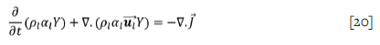
where a, is the volume fraction of the liquid phase in the mixture, p_l is the density of the liquid, Y is the mass fraction of the tracer species in the liquid phase, and J is the diffusion flux of the tracer species due to molecular and turbulent diffusion. The diffusion flux is obtained from the following equation:

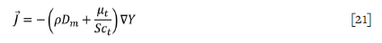
where D_m is the molecular diffusion coefficient for tracer species, Sc_t is the turbulent Schmidt number where μ is the turbulent viscosity), and D_t is the turbulent diffusivity. In this study the molecular diffusion is set to 2x10^-9m²/s and Sc_t is 0.7 (the default value in Ansys Fluent).

The properties of the tracer and the background liquid (water) are assumed to be identical. The concentration of the tracer will therefore not have any significant effect on the liquid flow field. In this case, the liquid flow equations (e.g. momentum and turbulence equations) and species equations are solved sequentially starting with the liquid flow solution. The tracer species equation is then solved as an unsteady simulation using the computed liquid flow solution.

Tracer injection and monitoring

The tracer is injected into the column using the pulse method. The tracer mass fraction at the column inlet is set to unity for time durations similar to the tracer injection time in the experimental column. In this case, the total injection time is i second for the industrial column, which was the value used in the work of Yianatos and Bergh (1992). After that, the mass fraction of the tracer is again set to zero and the simulations continued up to about 3600 seconds flow time. The mass fraction of the tracer is subsequently recorded at the outlet every 10 seconds and used to obtain the RTD curves from which the mean residence time (τ) and the vessel dispersion number (N_d) are calculated.

Particle age distribution and mean residence time simulation

The particle age distribution and mean residence time are modelled using a transport equation that computes the age (a_s) of the particles in the column. The particle age is defined as the time t that has elapsed since the particle's entry into the column such that a_s = t. This method has been applied in studies of mixing in different reactors in the chemical engineering field (Baléo and Le Cloirec, 2000; Baléo, Humeau, and Le Cloirec, 2001; Ghirelli and Leckner, 2004; Liu and Tilton, 2010; Simcik et al., 2012). However, this study is the first one to introduce particle age transport equations in column flotation modelling.

The introduction of the particle age equation offers an attractive method for predicting the solids mean residence time at lower computational cost compared with other methods that are based on Lagrangian particle tracking. In addition, the numerical solution of the particle age equations gives the distribution of particle (solids) residence time in the column, which can be used to understand the effect of liquid recirculation on the mixing behaviour of solids in column flotation.

In this method, the particle age a_s (or local residence time) is considered as a scalar property that is being transported by the particles. The rate of change of the particles age is therefore represented by the substantial (or convective) derivative as follows:

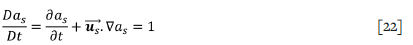
which is the advection equation for the scalar variable a_s. For the solid particles in the multiphase flow, the transport equation for the age of the particles (a) can be presented as follows:

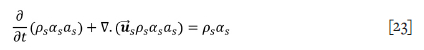
where a is the volume fraction of the solid phase (particles) while p_s is the density of the particles. This equation is introduced into the CFD model of the flotation column as a user-defined scalar (UDS) equation which is solved using the already computed velocity field of the solid phase. As for the boundary conditions, the particle age is set to zero at the inlet while a zero flux condition is specified for the particle age at the walls. On the other hand, the particle age at the outlet is extrapolated from the interior solution. The result is the spatial distribution of particle age in the column, which can be used to describe the mixing characteristics of the solid phase. The mean residence time of the solids (particles) is then obtained as the mass-weighted or area-weighted average age of the particles at the outlet of the column.

 

Results and discussion

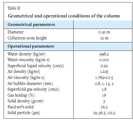
Three-phase CFD simulations were conducted to model the 0.91 m diameter cylindrical column that was used in the work of Yianatos and Bergh (1992). The operating conditions of the column are presented in Table II. Four different average bubble sizes, including 0.8, 1, 1.5, and 2 mm, were used in the simulations. The simulated RTDs obtained using the different bubble sizes were then compared in order to investigate the effect of bubble size on axial mixing in the column. For the validation of the model, results obtained from the simulations conducted with the 0.8 mm bubble size were compared with the experimental data. The 0.8 mm bubble size was used in the validation because that is the typical size of bubbles used in industrial flotation columns.

 

 

To simplify the CFD model and reduce the overall computational time, the bubble size is assumed to remain constant throughout the column. In reality, however, the size of the bubble will vary throughout its upward trajectory in the column because of the decrease in hydrostatic pressure, which will cause the bubbles to expand. This expansion of bubbles is the reason for the increase in gas holdup observed along the height of industrial flotation columns.

For the simulation of particles, the CFD simulations in this study were conducted using average particle sizes that fall within the range of sizes studied in the corresponding experimental work. Separate simulations were performed for each particle size in order to simplify the model and minimize the computational cost of the simulations. Possible effects of particle size distribution on the hydrodynamics of the column were therefore not captured in this study. The results obtained from the CFD simulations are presented below.

CFD simulation results

CFD simulations were conducted to model the cylindrical industrial flotation column that was used in the work of Yianatos and Bergh (1992). Their work involved measurement of both solids and liquid RTDs in the 0.91 m diameter column using radioactive tracer techniques. For the solids, RTDs were measured for three size classes; fine (-39 μιη), medium (-75+38 μιη), and coarse (-150+75 μιη). However, it is not the aim of the present research to simulate the entire particle size distribution in the column. The present study therefore uses three average particle sizes to represent each of the three size classes present in the column, namely; 19, 56.5, and 112.5 μ"¹. In addition, the subsequent

CFD simulations were performed with one particle size at a time in order to simplify the model further.

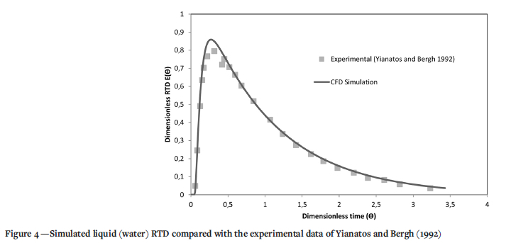
Liquid residence time distribution (RTD) The simulated liquid RTD is compared with the measured one in Figure 4. Since the particle size in the industrial column was predominantly less than 25 μm, the CFD simulation performed with 19 μm particle size is the one that is compared with the measured liquid RTD data. It can be seen that the CFD results are in good agreement with the measured liquid RTD.

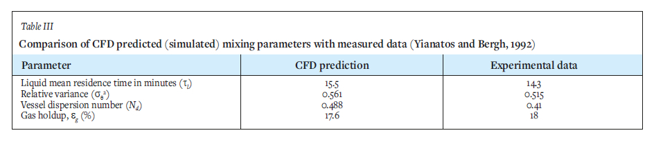
The mixing parameters (liquid mean residence time and vessel dispersion number) calculated from the CFD-simulated liquid RTD, together with the predicted air holdup, is compared with the values reported by Yianatos and Bergh (1992) in Table III. It can be seen that the simulated mixing parameters are in reasonable agreement with the literature data.

Effect of particle size and bubble size on liquid axial mixing

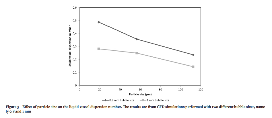
The effect of particle size on the liquid vessel dispersion number was investigated using liquid RTDs obtained from CFD simulations performed with different particle sizes. The results are shown in Figure 5 for simulations conducted with two different bubble sizes; 0.8 and 1 mm. It can be seen that increasing the particle size results in a decrease in the liquid vessel dispersion number. On the other hand, previous researchers have reported that the liquid vessel dispersion number (i.e., the liquid mixing intensity inside the column) decreased with increasing solids percentage (wt%) in the feed (Finch and Dobby, 1991; Laplante, Yianatos, and Finch, 1988; Xu, 1990). Subsequently, the feed solids percentage has been included in the empirical correlations that are used for estimating the vessel dispersion number for predicting the recovery in column scale up procedures. However, the effect of the particle size on the liquid vessel dispersion number observed in the present research suggests that particle size should also be considered in the correlations for estimating the vessel dispersion number in order to obtain correct predictions of the mineral recovery.

Figure 5 also shows that an increase in the bubble diameter reduces the liquid dispersion in the column. A similar result was reported by Xia, Peng, and Wolfe (2006), who observed that a reduction in bubble size resulted in a rise in the axial liquid velocity. The increase in liquid back-mixing can be attributed to the increase in gas holdup resulting from the reduction in bubble size. As the bubble size is reduced, the number of bubbles increases while the bubble rise velocity reduces, causing an increase in bubble residence time. The subsequent increase in gas holdup results in higher axial liquid velocity which will cause a stronger back-mixing effect (Xia, Peng, and Wolfe, 2006; Laplante, Yianatos, and Finch, 1988).

Particle (solids) mixing characteristics

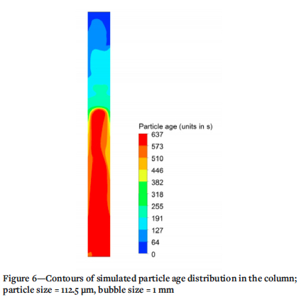
Solving the transport equation of the particle age in the column gives the spatial distribution of the age of the particles in the collection zone of the column. The contour plot of the spatial age distribution of 112.5 _um particles at the vertical mid-plane position in the column is presented in Figure 6 for illustration. The simulated particle age seems to increase from the walls towards the centre of the column. This is a result of the liquid circulation pattern in which the liquid (water) rises in the centre of the column and descends near the walls.

 

 

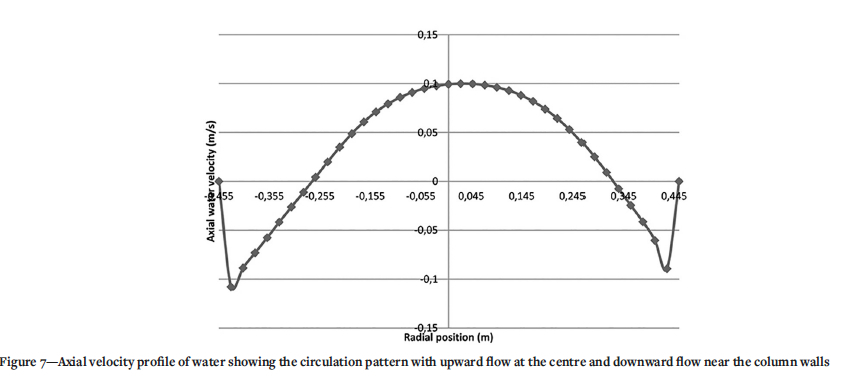
The effect of liquid circulation on particle age distribution in the column can be understood by examining the axial velocity profile of water presented in Figure 7. The velocity profile was obtained at the mid-height position in the column. It can be seen that the velocity is positive in the centre and negative near the walls of the column. The water is therefore rising in the centre and descending at the walls. The rising water carries with it 'older' particles that had reached the bottom part of the column while the descending water carries with it the 'younger' particles entering the column at the top. The particle age distribution in the column is therefore governed by the established liquid circulation prevailing in the column. These observations have important implications for the metallurgical performance of flotation columns because the back-mixing effect resulting from liquid circulation in the column might cause short-circuiting of feed to gangue flow, as earlier suggested by Xia, Peng, and Wolfe (2006). Gangue might also flow back to feed or concentrate flow and thus make separation less selective.

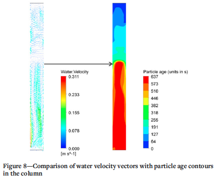
From Figure 6 it can be seen that the maximum particle age (red colour) is 637 seconds, i.e., about 10.6 minutes. However, the 'oldest' particles in the column are not only found at the outlet but also up to the middle height along the column. This can also be attributed to the liquid circulation pattern established in the column, in which the water rises in the centre of the column and descends near the column walls. The 'older' particles that reach the bottom are therefore lifted with the rising flow up to the middle part of the column. To verify this, the water velocity vectors were compared with the particle age contours in the column, as shown in Figure 8. The figure clearly demonstrates that the greatest particle ages (red contours) indeed coincide with two large liquid circulation cells occupying the bottom half of the column. This confirms the influence of the liquid recirculation on the particle age distribution inside the column.

 

 

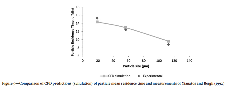
The particle mean residence time can also be obtained from the simulated particle age distribution and is given by the area-weighted average or mass-weighted average age of the particles at the outlet of the column. In Figure 9, the predicted particle mean residence times are compared with the experimental values reported by Yianatos and Bergh (1992). The mean absolute relative error (MARE) between the CFD predictions and the experimental data was calculated from the following equation:

With MARE equal to 7% the CFD results compared well with the experimental data.

The simulation results in Figure 9 also show that the solids (particle) mean residence time decreases with increasing particle size. This can be explained by the higher settling or terminal velocity of the larger solid particle in the presence of buoyancy. As the settling velocity depends directly on the diameter of particles, the solid particles of larger diameter experience faster downward motion toward the bottom of the column. Moreover, they have a higher probability of being caught in the downward liquid flow leading to the bottom of the tank. Thus, when solving the particle age equation for them they are less likely to stay longer within the tank. This is also evident in the corresponding experimental data. In comparison with the simulated liquid mean residence time of 15.5 minutes (refer to Table III), the predicted mean residence time of 9.6 minutes for the largest particle size (112.5 I™) was at least 60% of the liquid residence time. On the other hand, the smallest particle size (19 μm) had mean residence time (14.35 minutes) similar to the liquid one.

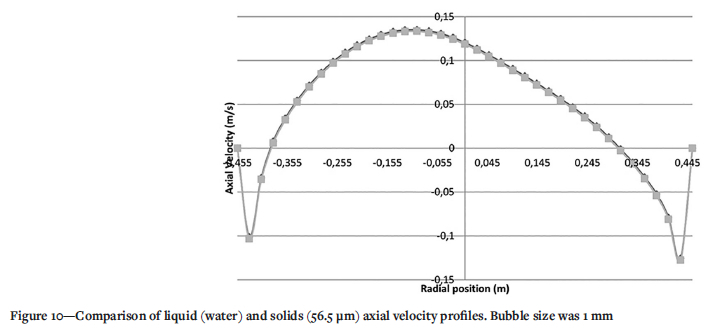
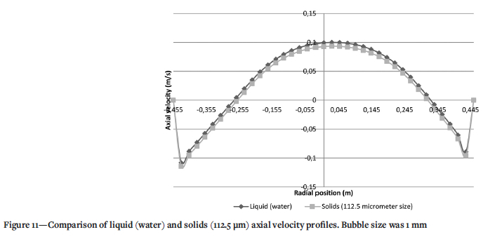
Equivalence of liquid and solids axial dispersion coefficients

Some previous researchers (Dobby and Finch, 1985; Yianatos and Bergh, 1992; Yianatos et al., 2005) have studied the relationship between the solids and liquid dispersion in column flotation and concluded that the solids vessel dispersion number (or axial dispersion coefficient) and the liquid one were equal. The solids mixing characteristics can therefore be estimated from the liquid axial dispersion coefficient for column scale-up and design purposes. However, the equivalence of the solids and liquid dispersion has been questioned by other authors citing various reasons (Goodall and O'Connor, 1991; Ityokumbul, 1992; Mills and O'Connor, 1990).

To clarify the relationship between the liquid and solids dispersion characteristics, the simulated liquid and solids (56.5 and 112.5 pm) axial velocity profiles at mid-height location are compared in Figure 10 and Figure 11. It can be seen that the solids axial velocities are similar to the liquid ones, even for the 112.5 pm particle size. The assumption of equal solids and liquid dispersion would therefore be applicable for normal operating conditions in an industrial flotation column.

Some researchers who have challenged the assumption of equal liquid and solids dispersion coefficients have argued that the solids content (3 wt%) used in the research that led to this conclusion was too small to highlight any differences between the two phases (Goodall and O'Connor, 1991). On the other hand, the solids content (16.2 wt% solids) in the present simulations was much higher than the 3 wt% referred to by Goodall and O'Connor (1991). It therefore seems reasonable for column flotation design and scale-up purposes to assume the equality of the liquid and solids axial dispersion coefficients.

 

Conclusion

In this research, the mixing characteristics of the liquid and solid phases in industrial flotation columns have been studied using computational fluid dynamics (CFD). The CFD results agreed favourably with the experimental data available from the literature. The results obtained showed that particle residence time decreases with increasing particle size. The residence time of the coarser particles (112.5 um) was found to be at least 60% of that for the liquid, while the finer particles (19 pm) had a residence time similar to that of the liquid.

The research further investigated the effect of bubble and particle sizes on the mixing characteristics of flotation columns. An increase in axial mixing in the column was observed when the bubble size was decreased. On the other hand, increasing particle size resulted in a decrease in the axial dispersion coefficient.

Another notable finding was the effect of the liquid recirculation on particle residence time in the column. It was established that the liquid flow pattern determines particle age distribution inside the column. Particle residence time distribution is therefore affected by liquid recirculation in the column.

The equivalence of the liquid and solids axial dispersion coefficients (or vessel dispersion numbers) was also investigated by comparing the water and the solids axial velocity profiles. The axial velocities of the two phases were found to be similar. It is therefore reasonable to assume equality of the solids and liquid dispersion coefficients for column design and scale-up purposes.

One of the limitations of this work is that the CFD simulations were performed using one particle size at a time. Any possible effects of particle size distribution on the hydrodynamics of the column are therefore not captured in the simulations. Future studies that incorporate population balance models or other means of incorporating particle size distribution are therefore recommended in order to further understand the mixing behaviour of solids in industrial flotation columns.

 

Nomenclature

DAxial dispersion coefficient, length2/time

CConcentration

C_DDrag coefficient

Drag force between phases p and q, N/m³

K_pqExchange coefficient in the momentum equation

External body force for phase q in the momentum equation (N/m³)

Gravitational acceleration, 9.81 m/s²

HHeight of the collection zone, m

Lift force in the momentum equation ((N/m³)

uLiquid interstitial velocity or particle velocity, m/s

YMass fraction of tracer species in the species transport equation

S_tMass source term for phase q, kg/m³s

a_sParticle age, s

Particle velocity vector, m/s

d_pParticle/bubble diameter, m

ReReynolds number (dimensionless)

Δt Time interval, s

tTime, s

kTurbulent kinetic energy, m²/s²

u_q Velocity of phase q, m/s

N_d Vessel dispersion number (dimensionless)

F_mqVirtual mass force in the momentum equation (N/m³) Greek letters

ρ Density, kg/m³

e_gGas (air) holdup

τ Mean residence time

σ_θ² Relative variance

Stress-strain tensor for phase q

â Turbulent dissipation rate, m²/s³

μ Turbulent viscosity, kg/m-s

σ² Variance

μ Viscosity, kg/m-s

aVolume fraction

Subscripts

GGas phase

lLiquid phase

PParticle/bubble

qPhase

sSolid phase

 

Acknowledgements

The authors would like to acknowledge the Centre for International Cooperation at VU University Amsterdam (CIS-VU) and the Copperbelt University (CBU) for providing the scholarship and subsequent funding for this research through the Nuffic-HEART Project. We would also like to acknowledge the Process Engineering Department and Rhasatsha High Performance Computing (HPC) cluster at Stellenbosch University.

 

References

Ansys Inc. 2013. ANSYS Fluent Theory Guide. Canonsburg, PA.         [ Links ]

Baléö, J.N. and Le Cloirec, P. 2000. Validating a prediction method of mean residence time spatial distributions. AIChE journal, vol. 46, no. 4. pp. 675-683.         [ Links ]

Baléo, J.N., Hümeaü, P., and Le Cloirec, P. 2001. Numerical and experimental hydrodynamic studies of a lagoon pilot. Water Research, vol. 35, no. 9. pp. 2268-2276.         [ Links ]

Chakraborty, D., Güha, M., and Banerjee, P. 2009. CFD simulation on influence of superficial gas velocity, column size, sparger arrangement, and taper angle on hydrodynamics of the column flotation cell. Chemical Engineering Communications, vol. 196. pp. 1102-1116.         [ Links ]

Deng, H., Mehta, R.K., and Warren, G.W. 1996. Numerical modeling of flows in flotation columns. International Journal of Mineral Processing, vol. 48, no. 1. pp. 61-72.         [ Links ]

Dobby, G.S. and Finch, J.A. 1985. Mixing characteristics of industrial flotation columns. Chemical Engineering Science, vol. 40, no. 7. pp. 1061-1068.         [ Links ]

Finch, J. A. and Dobby, G.S. 1990. Column Fflotation.Pergamon Press, Oxford.         [ Links ]

Finch, J.A. and Dobby, G.S. 1991. Column flotation: A selected review. Part I. International Journal of Mineral Processing, vol. 33, no. 1. pp. 343-354.         [ Links ]

Ghirelli, F. and Leckner, B. 2004. Transport equation for the local residence time of a fluid. Chemical Engineering Science, vol. 59, no. 3. pp. 513-523.         [ Links ]

Goodall, C.M. and O'Connor, C.T. 1991. Residence time distribution studies in a flotation column. Part 1: The modelling of residence time distributions in a laboratory column flotation cell. International Journal of Mineral Processing, vol. 31, no. 1. pp. 97-113.         [ Links ]

Harach, P.L., Waites, D.B., and Redfearn, M.A. 1990. Sparging system for column flotation. US patent no. 4,911,826.         [ Links ]

Ityokumbul, M.T. 1992. A new modelling approach to flotation column desing. Minerals Engineering, vol. 5, no. 6. pp. 685-693.         [ Links ]

Ityokumbul, M.T., Kosaric, N., and Bulani, W. 1988. Parameter estimation with simplified boundary conditions. Chemical Engineering Science, vol. 43, no. 9. pp. 2457-2462.         [ Links ]

Koh, P.T., Manickam, M., and Schwarz, M. 2000. CDF simulation of bubble-particle collisions in mineral flotation cells. Minerals Engineering, vol. 13, no. 14-15. pp. 1455-1463.         [ Links ]

Koh, P. and Schwarz, M. 2006. CFD modelling of bubble-particle attachments in flotation cells. Minerals Engineering, vol. 19. pp. 619-626.         [ Links ]

Koh, P. and Schwarz, M. 2009. CFD models of Microcel and Jameson flotation cells. Proceedings of the 7th International Conference on CFD in the Minerals and Process Industries. [CD-ROM] CSIRO, Melbourne:        [ Links ]

Kolev, N.I. 2005. Multiphase Flow Dynamics 2: Thermal and Mechanical Interactions. (2nd edn. Vol. 2. Springer, Berlin.         [ Links ]

Laplante, A.R., Yianatos, J.B., and Finch, J.A. 1988. On the mixing characteristics of the collection zone in flotation columns. Column Flotation '88. SME Annual Meeting, (pp. 69-80). Phoenix, AZ. I Sastry K.V. (ed.), pp. 69-80.         [ Links ]

Levenspiel, O. 1972. Chemical Reaction Engineering. (2nd edn). Wiley, Hoboken, NJ.         [ Links ]

Liu, M. and Tilton, J.N. 2010. Spatial distributions of mean age and higher moments in steady continuous flows. AIChE Journal, vol. 56, no. 10. pp. 2561-2572.         [ Links ]

Liu, T. and Schwarz, M. 2009. CFD-based multiscale modelling of bubble-particle collision efficiency in a turbulent flotation cell. Chemical Engineering Science, vol. 64, no. 24. pp. 5287-5301.         [ Links ]

Lun, C.K., Savage, S.B., Jeffrey, D.J., and Chepurniy, N. 1984. Kinetic theories for granular flow: Inelastic particles in couette flow and slightly inelastic particles in a general flow field. Journal of Fluid Mechanics, vol. 140. pp. 223-256.         [ Links ]

Mills, P.J. and O'Connor, C.T. 1990. The modelling of liquid and solids mixing in a flotation column. Minerals Engineering, vol. 3, no. 6. pp.567-576.         [ Links ]

Mills, P.J., Yianatos, J.B., and O'Connor, C.T. 1992. The mixing characteristics of solid and liquid phases in a flotation column. Minerals Engineering, vol. 5, no. 10. pp. 1195-1205.         [ Links ]

Mwandawande, I. 2016. Investigation of the gas dispersion and mixing characteristics in column flotation using computational fluid dynamics (CFD). PhD thesis, Process Engineering Department, Stellenbosch University, Stellenbosch, South Africa.         [ Links ]

Mwandawande, I., Akdogan, G., Bradshaw, S.M., Karimi, M., and Snyders, N. 2019. Prediction of gas holdup in a column flotation cell using computational fluid dynamics (CFD). Journal of the Southern African Institute of Mining and Metallurgy, vol. 119. pp. 81-95.         [ Links ]

Nadeem, M., Ahmed, J., and Chughtai, I.R. 2006. CFD-based estimation of collision probabilities between fine particles and bubbles having intermediate Reynolds number. Proceedings of the Fifth International Conference on CFD in the Process Industries. CSIRO, Melbourne.         [ Links ]

O'Connor, C.T. and Mills, P.J. 1990. The modelling of liquid and solids mixing in a flotation column. Minerals Engineering, vol. 3, no. 6. pp. 567-576.         [ Links ]

Rehman, A., Nadeem, M., Zaman, M., and Nadeem, B.A. 2011. Effect of various baffle designs on air holdup and mixing in a flotation column using CFD. Proceedings of the 8th International Bhurban Conference on Applied Sciences & Technology. Islamabad.         [ Links ]

Sarhan, A.R., Naser, J., and Brooks, G. 2016. CFD simulation on influence of suspended solid particles on bubbles' coalescence rate in flotation cell. International Journal of Mineral Processing, vol. 146. pp. 54-64.         [ Links ]

Shih, T.H. 1997. Some developments in computational modeling of turbulent flows. Fluid Dynamics Research, vol. 20. pp. 67-96.         [ Links ]

Simcik, M., Ruzicka, M.C., Mota, A., and Teixeira, J.A. 2012. Smart RTD for multiphase flow systems. Chemical Engineering Research and Design, vol. 90, no. 11. pp. 1739-1749.         [ Links ]

Wen, C.Y. and Yu, Y.H. 1966. Mechanics of Fluidization. Chemical Engineering Progress Symposium Series, vol. 62. pp. 100-111.         [ Links ]

Wheeler, D.A. 1985. Column flotation - The original column. Froth Flotation, Proceedings of 2nd Latin American Congress on Froth Flotation, Concepci6n, Chile..Castro, S.H. and Alvarez, J. (eds). Elsevier. pp. 19-23.         [ Links ]

Xia, Y.K., Peng, F.F., and Wolfe, E 2006. CFD simulation of alleviation of fluid back mixing by baffles in bubble column. Minerals Engineering, vol. 19, no. 9. pp. 925-937.         [ Links ]

Xu, M. 1990. Radial gas holdup profile and mixing in the collection zone of flotation columns. PhD thesis, Department of Mining and Metallurgical Engineering, McGill University, Montreal, Canada.         [ Links ]

Xu, M. and Finch, J.A. 1992. Solids mixing in the collection zone of flotation columns. Minerals Engineering, vol. 5, no. 9. pp. 1029-1039.         [ Links ]

Yianatos, J.B. and Bergh, L.G. 1992. RTD studies in an industrial flotation column: Use of the radioactive tracer technique. International Journal of Mineral Processing, vol. 36, no. 1. pp. 81-91.         [ Links ]

Yianatos, J.B., Bergh, L.G., Díaz, F., and Rodriguez, J. 2005. Mixing characteristics of industrial flotation equipment. Chemical Engineering Science, vol. 60, no. 8. pp. 2273-2282.         [ Links ] ♦

 

 

Correspondence:
G. Akdogan
Email: gakdogan@sun.ac.za

Received: 7 Apr. 2021
Revised: 24 Mar. 2022
Accepted: 31 Mar. 2022
Published: May 2022

 

 

ORCID: S.M. Bradshaw https://orcid.org/0000-0001-6323-8137
M. Karimi https://orcid.org/0000-0002-1182-1133
G. Akdogan https://orcid.org/0000-0003-1780-4075