PROFESSIONAL TECHNICAL AND SCIENTIFIC PAPERS

 

Mineral resource modelling using an unequal sampling pattern: An improved practice based on factorization techniques

 

 

D. Orynbassar; N. Madani

School of Mining and Geosciences, Nazarbayev University, Nur-Sultan city, Kazakhstan. N. Madani: https://orcid.org/0000-0002-5833-9758

Correspondence

 

 

---

SYNOPSIS

This work addresses the problem of geostatistical simulation of cross-correlated variables by factorization approaches in the case when the sampling pattern is unequal. A solution is presented, based on a Co-Gibbs sampler algorithm, by which the missing values can be imputed. In this algorithm, a heterotopic simple cokriging approach is introduced to take into account the cross-dependency of the undersampled variable with the secondary variable that is more available over the entire region. A real gold deposit is employed to test the algorithm. The imputation results are compared with other Gibbs sampler techniques for which simple cokriging and simple kriging are used. The results show that heterotopic simple cokriging outperforms the other two techniques. The imputed values are then employed for the purpose of resource estimation by using principal component analysis (PCA) as a factorization technique, and the output compared with traditional factorization approaches where the heterotopic part of the data is removed. Comparison of the results of these two techniques shows that the latter leads to substantial losses of important information in the case of an unequal sampling pattern, while the former is capable of reproducing better recovery functions.

Keywords: Co-Gibbs sampler, variogram analysis, data imputation, principal component analysis.

---

 

 

Introduction

Multivariate geostatistical analysis of cross-correlated variables is of paramount importance in orebody evaluation, which directly impacts further stages in a mining project such as resource classification, mine planning, and geometallurgical design (Battalgazy and Madani, 2019a, 2019b; Abildin, Madani, and Topal, 2019; Maleki et al., 2020; Adeli, Emery, and Dowd, 2018; Adeli and Emery, 2017, 2021). However, when the number of variables increases, the modelling process becomes cumbersome. This difficulty can be ascribed to two main factors. The first deals with establishing a linear model of coregionalization (Journel and Huijbregts, 1978) for the inference of the cospatial continuity (Leuangthong and Deutsch, 2003; Goovaerts, 1993). The second involves using a cokriging system for establishing and deriving the corresponding weights, which might be demanding in terms of computation time. This problem becomes more manifests when one is dealing with multivariate geostatistical simulation (Abildin, Madani, and Topal, 2019).

To overcome these impediments, several geostatistical avenues have been suggested in order to use factorization methods such as minimum/maximum autocorrelation factors (MAF) (Switzer and Green, 1985; Maleki and Madani, 2016), principal component analysis (Goovaerts, 1993), stepwise conditioning transformation (SCT) (Leuangthong and Deutsch, 2003), flow anamorphosis (Van den Boogaart, Mueller, and Tolosana-Delgado, 2017), and projection pursuit multivariate transform (Barnett, Manchuk, and Deutsch, 2016), to name a few. In these methods, the cross-correlated variables can be converted to uncorrelated factors where independent modelling can be implemented without the requirement to establish a cokriging system and infer a linear model of coregionalization. However, these approaches necessitate an equal sampling pattern of each variable, hence both variables should be accessible in all the sample observations. This, however, is problematic in the case of an unequal sampling pattern such as a partially heterotopic configuration (Wackernagel, 2003) of the data-set. One solution for using the factorization approach over such a data-set is to completely remove the incomplete part of the sample observations and continue the modelling process with the remaining isotopic portion of data. This could be problematic because one may lose a substantial part of the information (Barnet and Deutsch, 2015). Another alternative is to impute the values at unsampled locations to quantify the uncertainty, and then use the multivariate relationship that exist between the variables.

Methods and tools have been developed in this study first for data imputation at unsampled location by using a Co-Gibbs sampler algorithm in a multivariate case study, and secondly to use PCA for factorization of variables with imputed values for the purpose of mineral resource modelling.

We first review the theory of data imputation techniques. We then analyse the proposed data-set, apply data imputation techniques to the heterotopic data-set, and compare the results. Finally, we perform the resource modelling by PCA on the imputed data-set and original heterotopic data-set, and compare the results.

 

Methodology

Rationale of missing data

First, we consider the theory of missing data and basic concepts in this problem of geostatistical modelling. Missing data or incomplete data-sets do not necessarily imply flaws in the data collection process. A good example is in oil reservoir modelling, where there is always more seismic information available than other data (Xu et al., 1992). In this case, the abundance of secondary information can be used to improve the quality of estimation (modelling) using the scarce primary data alone. In ore deposits, it is also common to find a secondary variable that is abundantly available compared to the primary variable. The reasons for unequal sampling of the primary and secondary variables vary, but could be related to the costs of assaying some particular elements/minerals. In this sense, one may face three sampling patterns for the purpose of orebody evaluation in multielement deposits (Wackernagel, 2003) (Table I):

 

 

> Isotopic (homotopic): primary and secondary variables are available at all sample locations

> Totally heterotopic: primary and secondary variables are available at different sample locations

> Partially heterotopic: some primary and secondary variables share the same locations.

Most geostatistical algorithms need data at all sample locations (isotopic sampling). The challenge in geostatistical factorization analysis, therefore, is how to deal with the missing data in partially and totally heterotopic sampling patterns. An imprecise yet immediate solution is to remove the incomplete data from the whole data-set. However, losing this important information will produce biased results (Barnett and Deutsch, 2015). Another solution is using a regression function to impute the values at missing locations (Little and Rubin, 2002). For instance, linear regression analysis aims to fit a function to the available data irrespective of geographical location (Enders, 2010). This method is impractical since it provides a unique single value for that location where it is unable to compute the uncertainty. Another difficulty is that this method may ignore the location of the variables, and fail to recognize the spatial continuity of the corresponding variables. An alternative for data imputation is to simulate the values at unsampled locations by some iterative geostatistical approach such as the Gibbs sampler.

Gibbs sampler

The Gibbs sampler algorithm is a practical approach to missing data analysis (Barnett and Deutsch, 2015). The rationale of this algorithm is built on the Markov chain theory, which implements sampling from a multivariate Gaussian distribution. By virtue of its iterative nature, the Gibbs sampler updates the simulated values several times, taking into account the conditioning of available data, until it reaches a target distribution (Casella and George, 1992). In a univariate case, wherever only one variable is considered for imputation of the value at an unsampled location, a univariate Gaussian random vector with missed m observations, Z = (Z₁,..,Z_m)_r, with zero mean and variance-covariance matrix C, can be imputed in an iterative manner, by updating one selected observation based on conditioning to the other hard and previously imputed observations in the corresponding vector. This algorithm consists of the following steps (Barnett, Manchuk, and Deutsch, 2016; Madani and Bazarbekov, 2020):

> Initialization: Commence the imputation by an independent random vector Z⁽⁰⁾_mx1. This can be done by acceptance-rejection method.

> Iteration: for i = 1,2,...I

• Choose an index j e {1,.. .,m} either in regular or random order (Roberts and Sahu, 1997; Galli and Gao, 2001; Arroyo et al., 2012).

• Estimate Z_jconditionally to the other observations, (Z1,...,Z(j-1), Z(j+1),..Z_m) by employing simple kriging in a unique neighbourhood to return the kriging estimated value Z_j^sK(i)and variance of estimation error σ_j^SK(i). In this step, the conditioning data includes hard data and previously imputed values at missing n observations.

• Impute a new random vector Z_j⁽ⁱ⁾using the conditional distribution, with mean equal to its simple kriging estimate and variance equal to its variance of estimation error.

• Update the random vector by

• Go back to step 1 and loop I times.

One of the exceptional advantages of this sampling technique is the iterative process, i.e. it continues to simulate the values at undersampled points through a loop until it reaches the desired spatial continuity. The stated feature of the Gibbs sampler originates from the Markov chain that allows communicating of any states with positive probability distribution in a determined number of transitions, which accentuates the distinctive properties of this chain, namely aperiodicity and irreducibility (Lantuéjoul, 2002). Moreover, through promotion of the initial probability to a higher state, it aims at reaching the intended distribution (e,g. standard Gaussian distribution), which will entail the equilibrium or invariant distribution. These characteristics of the process encourage convergence of the global distribution to a Gaussian random vector with zero mean and the desired variance-covariance matrix C(x) through an increasing number of iterations (I_a) (Tierney 1994; Lantuéjoul 2002).

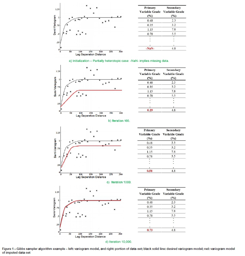
In order to illustrate the notation of the Gibbs sampler mechanism in data imputation, a simple example is provided. A data-set is given with N number of observations, including some missing observation locations (Figure 1a, right). The variogram model is constructed using the known (isotopic) part of the data and is depicted in Figure 1a, left. After running the Gibbs sampler with setting for 100 iterations, a value is inferred for the missing point (consider only one missing point), and the corresponding variogram is computed (Figure 1b, left). Subsequently, the results are given after 1000 and 10000 iterations (Figures 1c and 1d). With an increasing number of iterations, the variogram of the data-set, including the imputed value, approaches the variogram model, until it matches it completely, at which point the final value is accepted and iterations cease.

However, the Gibbs sampler algorithm is not suitable for multivariate data imputation, because it ignores the dependency of the undersampled variable on other available data. We now show how data imputation is performed in a multivariate context.

Proposed algorithm

In a multivariate data-set, the data imputation may result in total or partial heterotopic sampling patterns. In this method, the imputed values at missing locations are subject to the cross-correlation structure that exists between the primary and secondary variable. In this study, we only show the methodology for imputation in a multivariate case with a partially heterotopic sampling pattern. This can be applied further for resource modelling using the factorization techniques where an isotopic sampling pattern is required. Therefore, the first step is to impute the values at unsampled locations of the data-set to make the sampling pattern isotopic. In this respect the secondary variable with more data accessibility boosts the quality of imputation of values for the primary variable at missing locations. To achieve this, Madani and Bazarbekov (2020) proposed a Co-Gibbs sampler algorithm, in which simple kriging in the conventional Gibbs sampler (as already explained) can be substituted for the simple cokriging system based on two neighborhood search strategies:

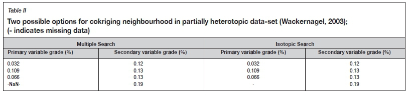
> Isotopic search: all sampling locations containing both the primary and secondary variables are selected (Table II, right).

> Multiple search: all sampling locations containing both the primary and secondary variables are selected, together with the secondary datum at target-undersampled location (Table II left).

These two neighbourhoods allow for two alternatives cokriging systems: (a) isotopic simple cokriging, and (b) heterotopic simple cokriging, in a unique neighbourhood. It is also possible to use moving neighbourhood; however, the rate of convergence may be slow and unconvincing (Arroyo, Emery, and Peláez, 2012). Readers are referred to Madani and Bazarbekov (2020) for more detail about the proposed Co-Gibbs sampler algorithm for data imputation.

Once both variables are available at sampling locations (i.e., building an isotopic sampling pattern), the next step is to decorrelate the variables. This can be done by any decorrelation technique; however, in this study we propose PCA due to its simplicity and straightforwardness. Since one avails several realizations at imputed locations, one needs to implement the PCA over all these realizations. In this step, one variable is always fixed and another variable that conveys the imputed values changes with each run of PCA. After this step, the factors can be simulated independently subject to the variogram analysis of each factor. Each realization of conditioning data leads to one realization over the target grids. Therefore, R realizations of imputed values produce R maps over the simulated grid nodes. Then, simulated results are back-transformed to the original scale to restitute the original correlation coefficient. The final step is to use the simulated results for resource modelling.

The capability of the proposed algorithm, its validity, and the improved performance of either of these two alternatives compared to the Gibbs sampler for data imputation, are presented and the proposed searching strategies are compared in the following case study.

 

Case study

The data-set used in this work belongs to an undisclosed gold deposit located in Australia. It includes 2458 sample locations with availability of two elements: gold (Au) and silver (Ag). This data-set is partially heterotopic, in that Ag data is less available and is missing at some sample locations, whereas Au grades are available at all sample locations. The 614 (scarce) Ag data points are primary, with the 2458 (abundant) Au data points being secondary. Therefore, only 614 observations include both Au and Ag variables (the isotopic part of the data-set).

Exploratory data analysis

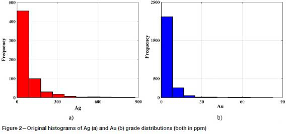
Exploratory data analysis establishes statistical parameters for the data-set aimed at detecting data errors and statistical inconsistencies which, if ignored, could lead to significant biases in the output results (Rossi and Deutsch, 2014). In this context, the presence of duplicates and outliers must be identified through diagrammatic statistical tools such as histograms and scatter plots, particularly in the case of s multivariate data-set (Rossi and Deutsch, 2014; Verly, 1993). Once identified, duplicate data and outliers are removed or capped from the data-set, respectively.

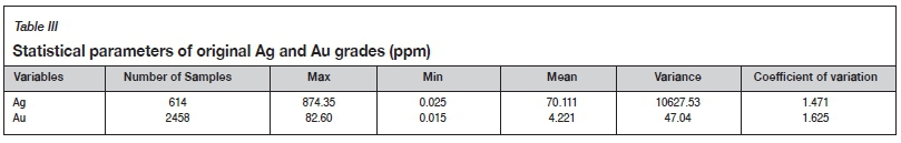
The original histograms for Au and Ag data are shown in Figure 2, and statistical parameters of the data-set are presented in Table III.

 

 

The linear correlation between the 614 isotopic silver and gold data-points, shown in the scattergram of Figure 3, has a correlation coefficient of 0.65, indicating a high dependency between Au and Ag in this deposit. The strength of the correlation coefficient suggests that data imputation by means of the proposed algorithm is acceptable, by first imputing values of Ag at locations missing this variable and secondly by apply PCA for Au resource modelling. The method is motivated because the Ag data will contribute to the modelling of Au in the deposit.

 

 

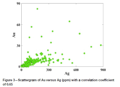
Generally, a high dependency between two variables and a heterotopic sampling pattern are two most important factors determining the suitability of the proposed algorithm in this study.

Normal score transformation and variogram analysis

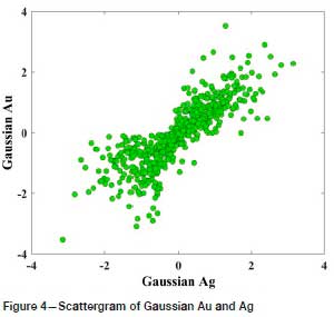
The first step in implementing the Gibbs sampler is a transformation of original data to a normal score distribution with mean 0 and variance 1, using an independent quantile-based approach for each variable (Verly, 1993). A scattergram of normal score-transformed data, shown in Figure 4, indicates a linear bivariate distribution of points, suggesting that the multivariate relationship between normal scores for Au and Ag meets bivariate Gaussianity.

 

 

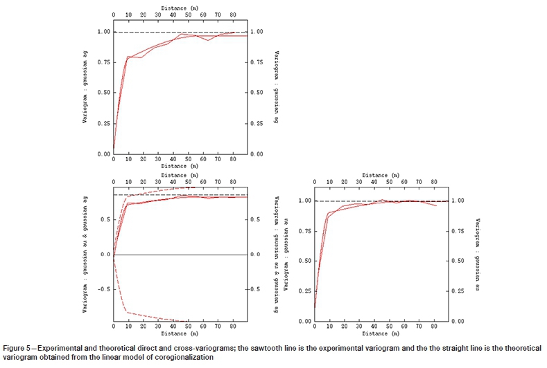
Next, the omnidirectional experimental direct and cross-variograms were calculated for the standard normal scores dataset. The cross-variogram is calculated for paired observations of silver and gold, i.e. the isotopic part of the data-set that involves only 25% of all the data. The variogram models were fitted by using the linear model of coregionalization, where a two-spherical structure, including the respective nugget effect, is fitted to these experimental variograms. The corresponding values of sill matrices, ranges, and models are as follow:

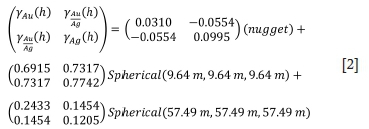
As can be seen in Figure 5, all depicted variogram models adequately reveal the spatial continuity of the data of interest. The sill variance for direct variograms has reached unity, entailing a stationary phenomenon. Lastly, the presence of a nugget effect (Equation [2]) also can be observed in all cases.

Results and validation

Once the linear models of coregionalization have been established, the Gibbs sampler algorithm can be implemented over the missing data locations to impute the Ag values. The number of iterations is set to 10 000, provided updates for inferred values can reasonably reach the target multivariate distribution.

Following the proposed algorithm, three alternatives of the proposed Gibbs sampler are mainly examined:

> GISO: Co-Gibbs sampler with isotopic simple cokriging.

> GHET: Co-Gibbs sampler with heterotopic simple cokriging

> GSK: Gibbs sampler with simple kriging

The results of two alternatives (GISO and GHET) are compared to the conventional Gibbs sampler where only simple kriging (GSK) is employed. Therefore, we consider this as the third alternative, where one ignores the existence of a secondary variable.

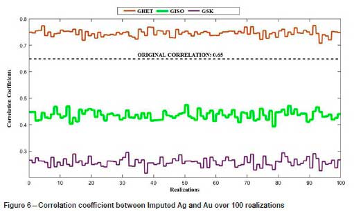
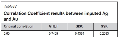
The derived results can be validated by examining the correlation coefficients between imputed Ag and Au values and comparing them with the original cross-correlation coefficient of 0.65. The distribution of correlation coefficients for 100 realizations is shown in Figure 6, with reference to the original correlation coefficient of 0.65. The average correlation coefficients for all three approaches, including GSK, are shown in Table IV. The overall outcome for the correlation between Au and imputed Ag values (GHET) is reasonably close to the original correlation coefficient (0.65), whereas GISO and GSK yielded poor results, failing to reach desired value of cross-correlation.

 

 

 

 

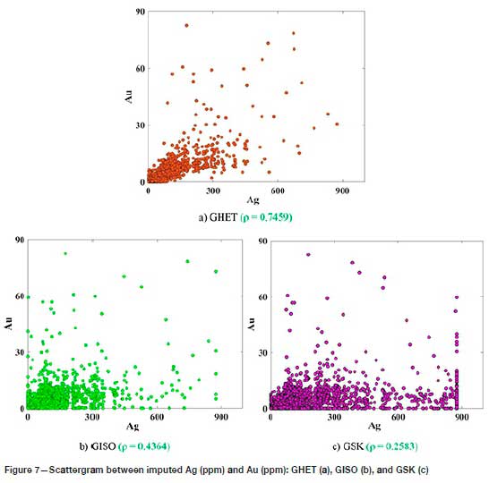
The measure of correlation between the average correlation of imputed values of Ag and original Au is another statistical parameter for validating the reproduction of bivariate relationships. A comparison of Figure 7 and Figure 3 shows that GHET outperformed GISO and GSK, the reason being that GISO and GSK ignore the importance of secondary data at the target locations. The efficiency of the Gibbs sampler alternative can be compared based on the reproduction of the original shape of bivariate relation (Figure 7). As can be observed, GSK's bivariate pattern certainly failed to follow the initial scatter pattern showing same value of Ag for a portion of the respective Au values. Also, from the visual representation of GISO's case, the pattern is ambiguous and does not properly reproduce the original 'diagonal' pattern. However, in the case of GHET, the bivariate relationship is compatible with the original bivariate relationship between Au and Ag, as demonstrated in Figure 3.

 

 

Resource calculation

The overall results show that the Gibbs sampler with heterotopic simple cokriging (GHET) provides satisfactory results in term of reproduction of original correlation coefficient for imputation of Ag values at missing sample locations.

Furthermore, through using available 100 series of the data-set, inclusive of the imputed Ag values, one can proceed to the resource calculation for the deposit. In this study, we chose principal component analysis (PCA) (Wackernagel, 2003; Sarma et al., 2007) for factorization of Au and Ag. The rationale/ principle of this methodology is to transform a set of correlated variables into independent uncorrelated factors thorough solving the eigenvalue problem.

The advantages of the proposed algorithm for resource modelling based on factorization by means of data imputation are considered in two cases:

> Case I: an isotopic sampling pattern for 614 sample locations where both Au and Ag are available

> Case II: an isotopic sampling pattern, where all 2458 sample locations are informed by existing Au data and imputed Ag values (100 realizations) obtained by heterotopic simple cokriging.

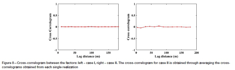
The first step after PCA factorization is to check the degree of correlation of derived factors at all lag distances. To achieve this, the cross-correlogram over the factors is calculated (Goovaerts, 1997) as illustrated for cases I and II in Figure 8, indicating the factors are uncorrelated over all lag distances. Therefore, one can use the independent simulation for modelling the factors since there is no dependency between these factors.

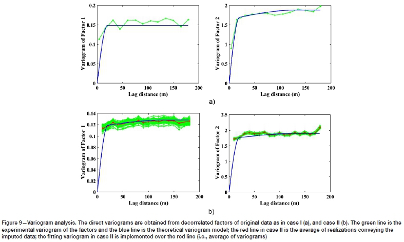
Variograms for the decorrelated variables of interest are established as a necessary step towards simulation. The variograms for case I and case II are illustrated in Figure 9. The variogram analysis for case II is implemented over the uncorrelated factors that are obtained from 100 imputed realizations for Ag. The average experimental variogram is calculated and the theoretical model fitted. The variogram formulae are as follows:

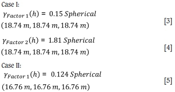
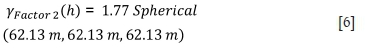
For both case, the variogram models are quite simple, consisting of only one structure (spherical) and without any nugget effects. Furthermore, case II with 100 realizations (green variograms) with averaged variogram (red variogram), and so the respective variogram fitting in case II was done over the average of variograms for simplicity.

Once the variogram models are derived, a turning bands simulation algorithm (Emery and Lantuejoul, 2006) is used to simulate the factors independently. This technique of simulation is selected because of simplicity and straightforwardness and its ability to reproduce the statistical parameters of the original data (Paravarzar, Emery, and Madani, 2015). The E-type maps (average map of 100 realizations/maps) of each case are illustrated in Figure 10. As can be seen, there is a visible difference between the results obtained from two cases.

 

 

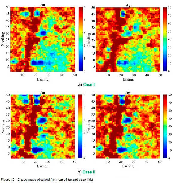
For instance, eastern part of the maps in Case II shows more concentration of both variables (Au and Ag) comparing to the maps obtained from Case I. This difference also is very tangible in the north-eastern and south-eastern part of the deposit. In north-eastern, Case I shows a high concentration of Au and Ag, whereas in south-eastern part of the region almost lacks the high concentration. This can happen due to ignoring substantial part of important information of Au by removing 1,844 sample observations in this Case. The results obtained from Case II is more compatible with the geological information of the deposit.

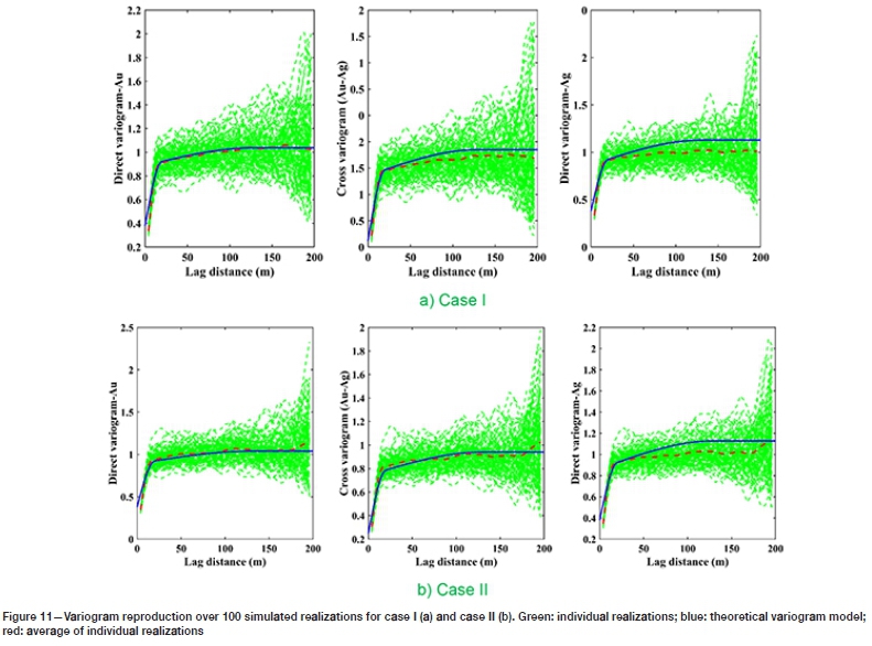
It is of interest to check which of the simulation results could produce the outcome approximate to the original statistical parameters of the data-set. The direct and cross-variograms for the simulation results can be compared with the original theoretical model, as shown in Figure 11. Cases I and II were both able to reproduce the spatial statistical parameters. The cross-variogram for case II is slightly better than that for case I, but not significantly so, since the cross-variogram is informed by homotopic part of the data-set (614 sample points), which is the same in both cases.

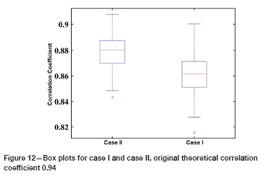
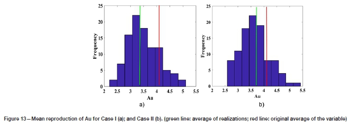
The box or whisker plot of the derived correlation coefficient distribution was calculated and is illustrated in Figure 12. Once again the findings from the imputed data-set are distinguished by a higher median value and shorter interquartile range (IQR) in case II. Reproduction of the mean value for Au is also examined through the calculation of a mean value for each of the 100 realizations, and the distribution of means is shown in Figure 13. As can be observed, case II improves the reproduction of the original mean.

 

 

The recovery functions, including tonnage, mean grade, and metal quantity above cut-offs for Au, are computed over the simulated results. As it can be seen from Table V, the results of the imputed data-set for case II provide the highest values of the recovery functions for each cut-off grade.

 

 

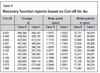
This significant difference should be seriously considered in the case of conventional removal of the data-set that is common in factorization techniques. Furthermore, the application of these methods goes beyond resource estimation, also affecting the cash flow of the project, the net present value (NPV) calculation, and other decision-making procedures in further mine planning exercises. Due to the distinct results obtained above, the data imputation role in enhancing the outputs should be reconsidered in modern resource modelling.

 

Conclusions

An iterative algorithm based on the Gibbs sampler has been presented in this study for data imputation at unsampled locations. For this, a heterotopic simple cokriging is applied in the Gibbs sampler that considers the cross-dependency of the undersampled variable with another variable that is more available. This algorithm showed that the correlation coefficient after imputation corresponds more closely to the original correlation coefficient. This shows that even using simple cokriging or simple kriging may not be an appropriate approach for such imputation. The results of employing a factorization approach also illustrate a good practice for resource modelling and calculation of recovery functions comparing to the traditional approaches, which only remove the incomplete part of the dataset, in terms of better computation of recovery functions. This work can also be expanded for modelling a data-set with more than two variables.

 

Acknowledgment

This research was funded by Nazarbayev University through the Faculty Development Competitive Research Grants for 2018 2020, grant number 090118FD5336. We are also grateful to the editorial team and two anonymous reviewers for their valuable comments, which substantially helped improving the final version of the manuscript. We also acknowledge Micromine Company for providing the data-set.

 

Computer code availability

The Co-Gibbs sampler executable file and the relevant source code files (Python-compatible) that are used in this study are freely available at https://github.com/btalgat/Co-Gibbs_Sampler/

 

References

Abildin, Y., Madani, N., and Topal, E. 2019. A hybrid approach for joint simulation of geometallurgical variables with inequality constraint. Minerals, vol. 9, no. 24. https://doi.org/10.3390/min9010024        [ Links ]

Adeli, A. and Emery, X. 2017. A geostatistical approach to measure the consistency between geological logs and quantitative covariates. Ore Geology Reviews, vol. 82. pp.160-169.         [ Links ]

Adeli, A. and Emery, X. 2021. Geostatistical simulation of rock physical and geochemical properties with spatial filtering and its application to predictive geological mapping. Journal of Geochemical Exploration, vol. 220. 106661.         [ Links ]

Adeli, A., Emery, X., and Dowd, P. 2018. Geological modelling and validation of geological interpretations via simulation and classification of quantitative covariates. Minerals, vol. 8. 7 pp. https://doi.org/10.3390/min8010007        [ Links ]

Arroyo, D., Emery, X., and Pelaez, M. 2012. An enhanced Gibbs sampler algorithm for non-conditional simulation of Gaussian random vectors. Computers & Geosciences, vol 46. pp. 138-148.         [ Links ]

Barnett, K.M. and Deutsch, C. 2015. Multivariate imputation of unequally sampled geological variables. Mathematical Geosciences, vol. 47. pp. 791-817.         [ Links ]

Barnett, K.M., Manchuk, J.G.m and Deutsch, C.V. 2016. The projection-pursuit multivariate transform for improved continuous variable modeling. SPE Journal, vol. 21. pp. 2010-2026.         [ Links ]

Battalgazy, N. and Madani, N. 2019a. Categorization of mineral resources based on different geostatistical simulation algorithms: A case study from an iron ore deposit. Natural Resources Research, vol. 28. pp. 1329-1351.         [ Links ]

Battalgazy, N. and Madani, N. 2019b. Stochastic modeling of chemical compounds in a limestone deposit by unlocking the complexity in bivariate relationships. Minerals, vol. 9. p. 683. https://doi.org/10.3390/min9110683        [ Links ]

Casella, G. and George, E.I. 1992. Explaining the Gibbs sampler. American Statistician, vol. 46. pp. 167-174.         [ Links ]

Emery, X. and Lantuéjoul, C. 2006. Tbsim: A computer program for conditional simulation of three-dimensional gaussian random fields via the turning bands method. Computers & Geosciences, vol. 32. pp. 1615-1628.         [ Links ]

Enders, C.K. 2010. Applied Missing Data Analysis, Guilford Press, New York.         [ Links ]

Galli, A. and Gao, H. 2001. Rate of convergence of the Gibbs sampler in the Gaussian case. Mathematical Geology, vol. 33. pp. 653-677.         [ Links ]

Goovaerts, P. 1993. Spatial orthogonality of the principal components computed from coregionalized variables. Mathematical Geology, vol. 25. pp. 281-302.         [ Links ]

Goovaerts, P. 1997. Geostatistics for Natural Resources Evaluation. Oxford University Press.         [ Links ]

Journel, A.G. and Huijbregts, C.J. 1978. Mining Geostatistics, Academic Press, London.         [ Links ]

Lantuéjoul, C. 2002. Conditional simulation of spatial stochastic models. Proceedings of ISMM2002I, Sydney, 3-5 April 2002. CSIRO Publishing, Clayton, Australia. pp. 327-335.         [ Links ]

Lantuéjoul, C. 2013. Geostatistical simulation: models and algorithms. Springer Science & Business Media.         [ Links ]

Leuangthong, O. and Deutsch, C.V. 2003. Stepwise conditional transformation for simulation of multiple variables. Mathematical Geology, vol. 35. pp. 155-173.         [ Links ]

Little, R.J. and Rubin, D.B. 2002. Statistical analysis with missing data. Wiley. New York.         [ Links ]

Madani, N. and Bazarbekov, T. 2020. An enhanced conditional Co-Gibbs sampler algorithm for data imputation. Computers & Geosciences, 104655.         [ Links ]

Maleki, M. and Madani, N. 2022. Multivariate geostatistical analysis: An application to ore body evaluation. Iranian Journal of Earth Sciences, vol. 8, no. 2. pp. 173-184.         [ Links ]

Maleki, Mohammad; Jélvez, Enrique; Emery, Xavier; Morales, Nelson. 2020. Stochastic open-pit mine production scheduling: A case study of an iron deposit. Minerals, 10, no. 7. https://doi.org/10.3390/min10070585        [ Links ]

Paravarzar, S., Emery, X., and Madani, N. 2015. Comparing sequential Gaussian and turning bands algorithms for cosimulating grades in multi-element deposits. Comptes Rendus Geoscience, vol. 347. pp. 84-93.         [ Links ]

Roberts, G.O. and Sahu, S.K. 1997. Updating schemes, correlation structure, blocking and parameterization for the Gibbs sampler. Journal of the Royal Statistical Society: Series B (Statistical Methodology), vol. 59. pp. 291-317.         [ Links ]

Rossi, M.E. and Deutsch, C.V. 2013. Mineral Resource Estimation, Springer Science & Business Media.         [ Links ]

Sarma, P., Durlofsky, L.J., and Aziz, K. 2008. Kernel principal component analysis for efficient, differentiable parameterization of multipoint geostatistics. Mathematical Geosciences, vol. 40. pp. 3-32.         [ Links ]

Sarma, P., Durlofsky, L.J., Aziz, K., and Chen, W.H. 2007. A new approach to automatic history matching using kernel PCA. Proceedings of the SPE Reservoir Simulation Symposium,, 2007. Society of Petroleum Engineers, New York.         [ Links ]

Switzer, P. and Green, A. 1984. Min/max autocorrelation factors for multivariate spatial imagery. Tech. Rep. 6. Department of Statistics, Stanford University.         [ Links ]

Tierney, L. 1994. Markov chains for exploring posterior distributions. Annals of Statistics. pp. 1701-1728.         [ Links ]

Van Den Boogaart, K.G., Mueller, U., and Tolosana-Delgado, R. 2017. An affine equivariant multivariate normal score transform for compositional data. Mathematical Geosciences, vol. 49. pp. 231-251.         [ Links ]

Verly, G. 1993. Sequential Gaussian cosimulation: a simulation method integrating several types of information. Proceedings of Geostatistics Troia'92. Springer.         [ Links ]

Wackernagel, H. 2013. Multivariate geostatistics: an introduction with applications, Springer Science & Business Media.         [ Links ]

Xu, W., Tran, T., Srivastava, R., and Journel, A.G.1992. Integrating seismic data in reservoir modeling: The collocated cokriging alternative. Proceedings of the SPE Annual Technical Conference and Exhibition, 1992. Society of Petroleum Engineers, New York.         [ Links ]

 

 

Correspondence:
N. Madani
Email: nasser.madani@nu.edu.kz

Received: 29 Aug. 2020
Revised: 8 Feb. 2021
Accepted: 29 Apr. 2021
Published: August 2021