PROFESSIONAL TECHNICAL AND SCIENTIFIC PAPERS

 

A new grade-capping approach based on coarse duplicate data correlation

 

 

R.V. Dutaut; D. Marcotte

École Polytechnique, Montreal, Quebec, Canada

Correspondence

 

 

---

SYNOPSIS

In most exploration or mining grade data-sets, the presence of outliers or extreme values represents a significant challenge to mineral resource estimators. The most common practice is to cap the extreme values at a predefined level. A new capping approach is presented that uses QA/QC coarse duplicate data correlation to predict the real data coefficient of variation (i.e., error-free CV). The cap grade is determined such that the capped data has a CV equal to the predicted CV. The robustness of the approach with regard to original core assay length decisions, departure from lognormality, and capping before or after compositing is assessed using simulated data-sets. Real case studies of gold and nickel deposits are used to compare the proposed approach to the methods most widely used in industry. The new approach is simple and objective. It provides a cap grade that is determined automatically, based on predicted CV, and takes into account the quality of the assay procedure as determined by coarse duplicates correlation.

Keywords: geostatistics, outliers, capping, duplicates, QA/QC, lognormal distribution.

---

 

 

Introduction

Outliers or extreme values are present in most mining grade data-sets. They can reflect true small-scale spatial variability and/or sampling and analytical errors introduced by procedures. Extreme values are deemed undesirable in kriging as they could propagate assay errors over significant ore tonnages. It is common practice in the mining industry to reduce these grade values to (or cap them at) a lower topcut value (Leuangthong and Nowak, 2015). Cap value determination is not straightforward and often remains subjective, especially for highly skewed distributions found in precious metal deposits.

Numerous methods have been proposed to address cap value determination, including the following:

➤Top percentile (Rossi and Deutsch, 2013): Most likely the simplest method, where the cap value is a high percentile of the distribution, generally between the 99th and 99.9th percentile. Sometimes the cap value is based on historical practices, such as capping at 1 ounce of gold per ton (this practice was common in northern Quebec, Canada). Although simple, the choice of cap percentile is arbitrary and subjective, and it does not take into account the quality of the assays.

➤Parrish capping (Parrish, 1997): The cap grade is selected such that the post-cap metal content of the assays above the 90th percentile represents less than 40% of the total metal and/or that of the assays above the 99th percentile represents less than 10% of the total. Although this method is repeatable, it can define overly conservative (i.e., very low) cap grades, especially for highly skewed deposits. In addition, the percentiles and the proportions used are arbitrary, and the method does not take into account the quality of the assay procedure.

➤Log probability (Rossi and Deutsch, 2013): A cumulative log probability plot, or more simply a data histogram, is used to identify a change in slope or a gap in the tail of the distribution. This is one of the most commonly used methods in the industry. It is relatively easy to interpret, but there are often multiple breaks/gaps in the distribution that make the choice of cap value subjective. In addition, the method is sensitive to the amount of data. For small data-sets, the cap value tends to be fairly low. When more data is available, the gap generally appears at a much higher value. The method also does not take into account the quality of the assay procedure.

➤Cutting curves (Roscoe, 1996): The average grade for different cap values is plotted and an inflection point is visually selected by the practitioner. This method is fairly arbitrary, and the choice of inflection point is subjective.

➤ Central variation error from the cross-validation of simulated local average (Babakhani, 2014): A local cap value is selected from a volume of influence (determined based on data spacing and kriging parameters) such that the interpolated block average within the volume is equal to the simulated median. A given high grade can be capped at different values depending on the neighbouring data. The method is complex as it requires kriging and conditional simulation, both of which need a variogram, on raw data for kriging and on Gaussian grades for simulation. The raw data variogram is itself sensitive to extreme values. The Gaussian transform required for simulation is also sensitive to extreme values. Furthermore, the results are likely to be sensitive to the choice of neighbourhood for both kriging and conditional simulation. In addition, this method requires coordinates, so it can't be used for conveyor, truck, or grab samples, for example.

➤ Metal risk analysis using simulations (Parker, reported in Rossi and Deutsch, 2013): Monte Carlo simulations are used to simulate the high-grade distribution. This method makes it possible to generate a confidence level for a predefined (e.g., yearly) metal production volume. This simulation method suffers from basically the same shortcomings as the method of Babakhani (2014).

It is worth noting that some authors have proposed alternative methods to avoid capping (David, 1977; Parker, 1991; Rivoirard, 2013; Maleki, Madani, and Emery, 2014). Although these methods are interesting from a theoretical point of view, they are rarely used in mining applications, where the capping of extreme values is still perceived as a best practice.

In this research, we propose the use of the correlation of the coarse duplicates to determine the cap value. The use of duplicates is now mandatory according to QA/QC guidelines and routine in the mining industry. Although Abzalov (2011) and Rossi and Deutsch (2013) describe various uses for duplicate samples, helping the determination of the cap level is not one of them. A rarely documented and supplementary question in resource assessments is whether capping should be performed before or after compositing.

Using a multiplicative lognormal error model, it is possible to determine the coefficient of variation of the true (unobserved) grades from the correlation between original and duplicate values (see later). We propose to determine the cap grade such that the newly capped population has the same CV as the CV determined from correlation between original and duplicate pairs.

After describing the multiplicative lognormal error model, the link between the lognormal parameters of the true grades, those of the errors, and the theoretical correlation between duplicates is derived. From this correlation, the predicted theoretical coefficient of variation of the grades is obtained and established as the target to be reached when determining the cap grade. The robustness to the sample length and the lognormal assumption is then assessed and the effects of capping before or after compositing is also analysed. Finally, case studies of a gold and a nickel deposit are presented, and cap grades obtained using the proposed approach are compared to those obtained using some traditional methods.

 

Methods

This section presents the multiplicative lognormal error model and the main results that are derived from it. Synthetic case studies are used to assess the method's robustness with regard to some assumptions and to measure the effects of capping before or after compositing.

Theoretical background

Assuming the following model (Marcotte and Dutaut, 2020) is valid:

where Z_ois the observed value at the x position, Z_vis the true value, and t is the multiplicative error of the analysis (in this study both Z_vand t are assumed to be lognormal, a reasonable assumption for most precious and base metal deposits). Equation [1] can be written:

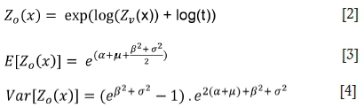
where α and β are the logarithmic mean and standard deviation of Z_vrespectively, and μand σ are the logarithmic mean and standard deviation of t respectively. Note that in the multiplicative lognormal error model, σ² is related to the variance of the duplicates' log-ratio:

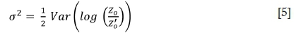
where Z₀and Z_o'are the observed original and duplicate assays (in short, duplicates values). Hence, σ² can be estimated directly from the duplicates independently of the other parameters (α, β, μ). This result is not used hereinafter but is presented for the sake of completeness.

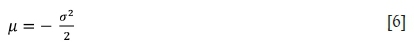
If quality assurance and quality control (QA/QC) is performed and sampling theory guidelines are followed, there should be no or limited bias on mean grade. From Equation [4] this implies:

Correlation between duplicates

The theoretical correlation between duplicates in the multiplicative model is given by:

The first equality comes from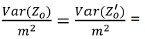

for the denominator and

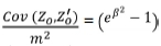
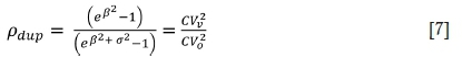
in the numerator. The last equality in Equation [7] comes directly from the definition of coefficient of variation and Equations [3] and [4] for the denominator and the same equations with σ²= 0, for the numerator. With σ² estimated from Equation [5] and correlation between duplicates, it is possible to estimate β using Equation [7] and then α using Equation [3]. Better yet, from Equation [7], the squared coefficients of variation of true and observed values are directly related to the duplicates' coefficient of correlation by:

where CV_vis the (unobserved) coefficient of variation of Z_vand CV_ois the (observed) coefficient of variation of Z_o. Hence, it is possible to estimate the coefficient of variation of the true grades using only the correlation between duplicates and CV_ocomputed with all available samples.

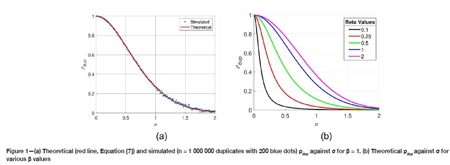
Figure 1a shows the curve defined by Equation [8], with β = 1, and simulated results. Figure 1b illustrates Equation [8] for different β values.

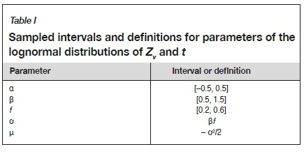
Figure 2 compares the theoretical error-free coefficient of variation defined by β to CV_predpredicted using duplicates correlation p_dup and CV_dupin Equation [8]. Each point represents a different lognormal distribution with parameters uniformly drawn in intervals described in Table I. As the number of duplicates increases, the spread of the points and the skewness of the conditional distribution of CV_predI CV_theo diminish. The number of duplicates required to estimate CV_theo to a given precision increases with CV value. Note that in Table I, the minimum and maximum theoretical CV are = 0.53 and = 2.91, which cover most practical cases. Also, σ < β and using Equation [8], the minimum and maximum theoretical p_dupare 0.42 and 0.957 respectively. Using Equations [3] and [4], the minimum and maximum theoretical CV_oare 0.54 and 4.51 respectively, which cover most practical cases.

 

 

Capping based on correlation between duplicates

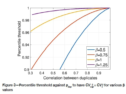
Equation [8] indicates that the coefficient of variation of the observed duplicate grades is inflated by sampling errors. This suggests the following capping criterion: choose the threshold providing CV_cap= CV_preddetermined experimentally from the correlation between duplicates and the coefficient of variation computed using all available samples (original and duplicates) using Equation [8]. This criterion, although arbitrary, has the advantage of being objective, repeatable, and simple to compute. It takes into account the quality of the assay procedure in determining the cap value, contrary to existing methods. Moreover, it does not require localization of the samples, contrary to the methods of Babakhani (2014) and Parker (1991).

Figure 3 shows the cap percentile applied to the distribution of Z_othat provides CV_cap= CV_predas a function of p_dupfor different values of β. All curves are computed by numerical integration of the truncated lognormal distribution. As expected, the cap percentile for each curve increases with the duplicates correlation, indicating that large error variances (lower duplicates correlation) require a lower cap value to obtain the desired coefficient of variation. Also, for a given correlation, the cap threshold increases with β, indicating a lower cap value is required for less skewed distributions of Z_v. Note that parameter α has no influence on determining the cap percentile.

 

 

Effects of variable assay supports

The results obtained so far assume the duplicate assays were on samples with identical supports. However, this might be not the case in practice for a variety of reasons (geological contacts, different sampling campaigns, technical drilling difficulties, etc.). It is therefore important to assess the effects of support variations on the statistics p_dupand β used to determine the cap percentile. Note that σ is the standard deviation of the error due to sample preparation and analysis; hence, it is not related to the support. Only β varies with the support.

If the point variogram is available, it is possible to compute the variance of the regularized support for any support. Assuming that distribution remains lognormal with the same mean, it is possible to compute ß_s, the logarithmic standard deviation associated with support s. The beta corresponding to a given support can be computed using classical geostatistical relations as:

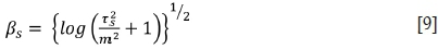
where is the logarithmic variance at point support, and γ (s,s) is the average variogram value within support s.

Example

Consider a typical gold deposit case with α = 0, β₀ = 1, the mean m = exp(0.5) = 1.65 ppm, the point true grade variance x₀ = m² (exp = 4.67 ppm² and a spherical variogram with correlation range 20 m. The assay supports are half cores of lengths varying between 1 m and 5 m. The corresponding variances of core grades are 4.5 ppm² and 4.1 ppm² for 1 m and 5 m lengths respectively, corresponding to β_1ηι= 0.99 and β_5ηι= 0.96. Further computing duplicates correlation using Equation [7] and σ = 0.5 for the two supports gives values of 0.69 and 0.68 respectively. Other values of σ provide similar differences in correlation and α has no impact on determining β and p_dup. As seen in this example, the effects of the support on β and p_dupare negligible when compared to the precision of the estimates of duplicates correlation and coefficient of variation.

Figure 3 indicates that realistic cap percentiles should be obtained for the lognormal case when the distributions are skewed (large β and CV) and the correlation between duplicates is high. when the skewness is low, the cap percentile tends to decrease, meaning that a significant percentage of the samples will be capped unless this is compensated for by a higher duplicates correlation corresponding to a better sampling preparation procedure in real deposits.

The lognormal assumption is realistic for many low-grade skewed distributions, which are typically encountered in precious- and base metal deposits. To get an idea of the sensitivity of the proposed approach to the lognormal assumptions, five different cases were simulated with a large quantity of data (1 million). Table II describes the five simulated cases. Figure 4 shows the duplicates' scattergrams and the histograms of the error-free simulated Z_vand the observed Z₀. Despite the strong departure from lognormality and small CV_v of each case, the five cap values determined by our approach appear reasonable in terms of percentile of the observed grades. Moreover, the CV of the capped values matches very well in each case with the CV of the error-free Z_v, indicating that Equation [8] also approximates the true CV in the non-lognormal case well.

Capping after or before compositing?

Some practitioners favour capping before compositing, others advocate doing so after. The argument of the 'before' camp is that possible outliers are averaged in the compositing process and can thus pass undetected, especially when the assay length is related to the presence or absence of visible mineralization. On the other hand, the 'after' camp maintains that assays over longer supports are already diluted, so it seems reasonable to dilute the outliers obtained on shorter supports to treat them like all other segments of the boreholes. But in fact, does it really matter?

A simple experiment

A series of synthetic boreholes totalling 300 000 m are simulated at every 10 cm. The variogram model is spherical with range 20 m. The distribution is lognormal with α = 0 and β = 1. Synthetic grades on variable lengths are computed according to the grade of the first 10 cm. The length is set to 0.5 m when Z(x) > (where Q90 is the quantile 0.9 of the simulated distribution), 3 m when v(X) > Q₇₅, and 1.5 m otherwise. This scenario mimics preferential sampling of visible mineralization. The 'true' assays Z_vare obtained on the specified lengths by averaging the simulated values. Then a multiplicative error t (drawn from a lognormal distribution with σ = 0.8) is applied to each assay to form the set of observed assays Z,.

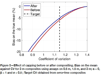
In the 'before' case, a series of potential cap values is applied to observed assay grades. Then regular 3 m composites are formed using the capped assays. In the 'after' case, the 3 m composites are formed using the raw assays and then the cap values are applied to the composites. The target CV_Vfor both cases is computed using the simulated Z_vat each 10 cm regularized over the variable length (in the 'before' case) or the composite length (in the 'after' case). Compositing is done on capped values for the 'before' case. The bias on mean in % (relative to simulated uncapped data) after capping the composites is computed. Results are shown in Figure 5. The 'after' case presents slightly less bias on the mean for any given CV_capthan the 'before' case. Similar results (not shown) were obtained for different cases by varying the composite lengths, the variogram range, and parameters α, β and σ.

 

 

Work flow

To summarize, we propose to apply the following work flow to objectively determine the cap value based on duplicates:

➤Compute correlation between coarse duplicates

➤Compute the observed coefficient of variation (CV₀) using all data available

➤Estimate CV_V, the target coefficient of variation of the error-free composites' grades, using Equation [8]

➤ Experimentally determine the cap value to apply to the composites to obtain CVcap = CV_V.

 

Case studies

In the following section, two real duplicate data-sets were used to compare the proposed capping strategy to some of the industry's most widely used methods.

Gold case

The first case study is on gold duplicates. Duplicate samples were obtained from 5 m blast-holes (diameter 96 mm) using sampling of the cuttings in the cone around the drill string. Sample preparation consisted of pre-crushing 5 kg of cuttings to 2 mm and then pulverizing 250 g to 75 μm. Fire assaying was done on 30 g aliquots with an atomic absorption (FA-AA) finish. The data-set contains 1 786 samples for a total of 3 572 duplicate assays. The gold duplicates' scattergram (Figure 6) shows ρ = 0.27 indicates an important overall sampling error. The artifact below 10^-2 for both duplicate assays reflects the limits of detection used by the assay laboratory. It is also seen in the spike at low levels in the probability plot. This low correlation is undesirable but sadly common in practice, especially in blast-hole samples. The log probability plot shows a gap in the upper tail around the 0.995 percentile value, which was retained as the log probability plot capping level.

Table III presents the cap results obtained using the different methods tested. The cap grades vary from 1.91 g/t to 4.49 g/t. The proposed method shows the second highest cap value at 3.69 g/t. The theoretical CV based on Equation [8] is 1.76. By design, the proposed method returns the same CV. The 99th percentile method returns the next closest one. The log probability plot and Parrish methods suggest cap values that result in a strong overestimation and underestimation, respectively, of the target CV value.

Nickel case

Drilling was done using the air core (AC) technique and 6 kg duplicates were created from the chips using a riffle splitter. Then 500 g of material were crushed to 2 mm and 250 g were pulverized to 75 pm. Fire assaying was done on 20 g aliquots with an XRF finish. The data-set contains 698 samples. Each sample provided two coarse duplicates for a total of 1396 duplicate assays.

The nickel duplicates present similar basic statistics (Figure 7), with a much lower kurtosis value than for the gold data-set. The high duplicates correlation coefficient (ρ = 0.94) indicates good reproducibility of the assays, as expected for a base metal deposit.

Table IV shows the cap results obtained using the different methods. The proposed method presents the highest recommended cap value as a result of strong duplicates correlation. All other methods underestimate the target CV (0.783), a consequence of selecting an overly low cap value.

 

Discussion

In mining applications, extreme values can often be encountered and must be controlled to avoid spreading high grade to large areas. The capping strategy can significantly impact the results of geostatistical and economic studies. In the exploration phase, an unduly low cap value can lead to an overly conservative resource estimate, possibly resulting in project rejection. On the other hand, too high a cap value may lead to an overly optimistic economic valuation and serious losses for mining companies. Various methods have been proposed in the past and are routinely used in the industry to determine cap values. Most are based on rather arbitrary empirical rules or on a subjective graphical interpretation of the cumulative distribution function. None use the important and mandatory coarse duplicate data to help determine a reasonable cap value that takes into account the quality of the assay procedure.

The proposed approach fills this gap. An unbiased multiplicative lognormal error model was used to derive the relationship between the observed and true grade CVs. The two CVs are simply linked through the duplicates correlation coefficient (see Equation [8]). One can predict the unobserved true CV from the observed CV with an estimate of the duplicates correlation. The proposed capping strategy is simple: select the cap value such that the CV of the capped samples is equal to the predicted true CV value.

Simulated data-sets showed that Equation [8] is unbiased for the true CV, even with a relatively small amount of duplicate data (Figure 2). They also showed that the analysed length has a limited impact on the proposed method, as both ρ and CV_o are relatively robust in response to this factor. Finally, Figure 4 illustrates the good stability of the method relative to different departures from the lognormal assumption.

The question of capping before or after compositing was also examined. Simulated data-sets with a preferential re-sampling approach (i.e., the intersections of high grade are analysed on shorter lengths than low grade) were used. The differences between the 'before' and 'after' cases are rather small but systematic. The 'before' case leads to more bias on the mean than the 'after' case for all CVs. We therefore recommend capping after compositing to minimize the bias on the mean.

The proposed approach was compared to some of the methods most widely used in the industry using two real data-sets, one for gold and the other for nickel, where coarse duplicates were available. With the proposed approach, the CV computed using capped data was equal to the predicted true CV by design. Interestingly, the proposed approach had the highest cap value of all the methods tested when reproducible duplicate data was available (nickel case, ρ = 0.94) but not for duplicate data with low correlation (gold case, ρ = 0.27). This illustrates that the capping strategy of the proposed method, contrary to other methods, takes into account the quality and reliability of assay data measured by duplicates correlation. Other advantages of the proposed approach are its simplicity and objectivity, as it can easily be computed automatically from assays and duplicate datasets without requiring variogram modelling, kriging, simulation, or cdf plotting and gap/break interpretation like some of the other methods.

When following QA/QC recommendations, thousands of duplicates are typically obtained even before the prefeasibility study. Hence, enough data is available to reliably estimate the correlation coefficient between duplicates. In earlier stages, when only a smaller quantity of duplicates is available, it might be interesting to consider a robust estimator of duplicates correlation. Many such robust estimators are described in the statistical literature. Further study is required to assess the influence of using different correlation robust estimators on the proposed method. Robust estimators of CV_ocould also be considered but this appears less necessary as much more data is available for CV_oestimation.

 

Conclusions

A new capping strategy based on the correlation coefficient between coarse duplicates is proposed. It incorporates the idea that the higher the correlation coefficient between duplicates, the greater the confidence level of the assay value, and accordingly the higher the cap value should be. The method proved to be robust to variations in sample support (assay length), departure from lognormality, and capping before or after compositing. When applied to gold and nickel deposit data, the proposed approach provided cap grades that reflected the reliability of the assays and were generally higher than those obtained with the other methods tested. The proposed approach is simple, objective, and repeatable. It makes it possible to automatically determine the cap grade from duplicate data.

 

References

Abzalov, M. 2011. Sampling errors and control of assay data quality in exploration and mining geology. Applications and Experiences of Quality Control. Intech Open.         [ Links ]

Babakhani, M. 2014. Geostatistical modeling in presence of extreme values. Master's thesis, University of Alberta, Canada.         [ Links ]

David, M. 1977. Geostatistical Ore Reserve Estimation. Elsevier.         [ Links ]

Leuangthong, O. and Nowak, M. 2015. Dealing with high-grade data in resource estimation. Journal of the Southern African Institute of Mining and Metallurgy, vol. 115, no. 1. pp. 27-36.         [ Links ]

Maleki, M., Madani, N., and Emery, X. 2014. Capping and kriging grades with long-tailed distributions. Journal of the Southern African Institute of Mining and Metallurgy, vol. 114, no. 3. pp. 255-263.         [ Links ]

Marcotte, D. and Dutaut, R. 2020. Linking Gy's formula to QA/QC duplicates statistics. Mathematical Geosciences. September. pp. 1-13, https://doi.org/10.1007/s11004-020-09894-x        [ Links ]

Parker, H. 1991. Statistical treatment of outlier data in epithermal gold deposit reserve estimation. Mathematical Geology, vol. 23. pp. 175-199.         [ Links ]

Parrish, O. 1997. Geologist's gordian knot: To cut or not to cut. Mining Engineering, vol. 49. pp. 45-49.         [ Links ]

Rivoirard, J., Demange, C., Freulon, X., Lécureuil, A., and Bellot, N. 2013. A top-cut model for deposits with heavy-tailed grade distribution. Mathematical Geosciences, vol. 45. pp. 967-982.         [ Links ]

Roscoe, W. 1996. Cutting curves for grade estimation and grade control in gold mines. Proceedings of the 98th Annual General Meeting, Edmonton, Alberta, 29 April. Canadian Institute of Mining, Metallurgy and Petroleum, Montreal.         [ Links ]

Rossi, M.E. and Deutsch, e.V. 2013. Mineral Resource Estimation. Springer Science & Business Media.         [ Links ] ♦

 

 

Correspondence:
R.V. Dutaut
Email: raphael.dut@wanadoo.fr

Received: 10 Sep. 2020
Revised: 14 Feb. 2021
Accepted: 18 Feb. 2021
Published: May 2021

 

 

R.V. Dutaut https://orchid.org/0000-0001-7474-2574
D. Marcotte https://orchid.org/0000-0002-5784-9115