DEEP MINING PAPERS

 

Addressing misconceptions regarding seismic hazard assessment in mines: b-value, M_max, and space-time normalization

 

 

J. Wesseloo

Australian Centre for Geomechanics, The University of Western Australia, Australia

Correspondence

 

 

---

SYNOPSIS

Seismic hazard assessment, in some form or another, has formed part of seismic risk management in seismically active hard-rock mines for decades. Some misconceptions, however, exist in the mining industry which may lead to errors in interpretation and poor risk management decisions. This paper addresses some misconceptions the author has encountered in the mining industry. This is done by exploring the meaning and implications of the frequency-magnitude distribution. The meaning of M_max, the methods of assessing it, and the topic of space and time normalization necessary for the evaluation of seismic hazard, are also addressed. The scope of this paper does not include the evaluation of strong ground motion exceedance which also forms part of the evaluation of seismic hazard at mine sites.

Keywords: Seismic risk, frequency-magnitute distribution, normalization probability.

---

 

 

Introduction

At any seismically active mine, considerable effort is invested into the effective management of seismic risk (see Potvin et al., 2019), of which seismic hazard assessment is, of course, a fundamental component. Over many years I have come across several misconceptions regarding the assessment of the seismic hazard which adversely affect the standard of seismic risk management in our industry. Some of these misconceptions are widespread and deeply rooted, while others crop up from time to time and seem to migrate through the industry. The aim of this paper is to address some of those misconceptions.

The frequency-magnitude (FM) distribution is foundational to understanding seismic hazard. It appears, however, that many of the misunderstandings regarding seismic hazard arise from inadequate understanding of the meaning and implications of the FM distribution. For this reason, a large proportion of this paper will be devoted to the FM distribution and its implications. The fact that 'M_max' is used for several different concepts, further creates confusion and misunderstanding. Another topic that does not seem to be well understood is that of normalization of hazard, with respect to space and time, and the related issue of separating sources of seismicity with different behaviour.

The assessment of seismic hazard in mines also includes the evaluation of strong ground motions at specific locations. This topic is, however, excluded from the scope of this paper.

 

What is the Gutenberg-Richter relationship really?

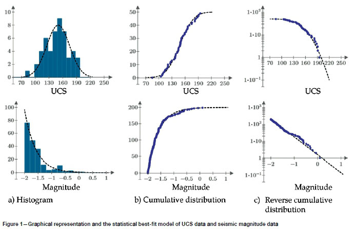
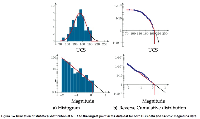
It appears that many misconceptions in the mining industry stem from an inadequate understanding of the FM distribution and its implications. Many rock engineers use the FM chart without realizing that it is simply a reverse cumulative distribution¹ of magnitude, with the vertical axis plotted on a log scale. The straight line fit, or any other curve fitted to the data, is therefore simply a statistical best-fit model and is conceptually the same as, for example, a normal distribution fitted to UCS data (see Figure 1).

The model most often used for seismic magnitude distribution is the Gutenberg-Richter (GR) relationship (Gutenberg and Richter, 1944):

Which we can write as:

where:

N is the number of events with magnitude > M

M is the event magnitude

a is the coefficient quantifying the number of events

b is the coefficient quantifying the log relative occurrence of smaller to larger events

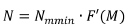
In the case of seismic magnitude data, however, limitations in the system sensitivity result in small events not being recorded. For statistical and probabilistic analysis, one can therefore only use the data above the magnitude of completeness, m_mln, with the statistical density and cumulative function being limited to the magnitude ranges greater than m_mn. We can write the GR relationship in Equation [2], with respect to the reverse cumulative distribution function, as follows:

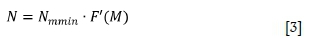
with

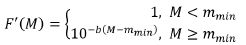
and

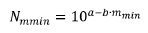
Where

N_mmnis the number of events with magnitude greater than m_mn F(M is the reverse cumulative distribution function

It is interesting to note that F(M) in Equation 2 is simply a different formulation of the commonly used negative exponential distribution, translated to start at m_mninstead of zero.

The open-ended GR relationship (Equations [1] and [2]) predicts a non-zero probability of physically impossible magnitude sizes, (i.e., the probability of a Richter magnitude > 10 is not zero!). For this reason, equations that truncate at large magnitudes are preferred, for which several different relationships have been proposed (Utsu, 1999). In mining, the truncated Gutenberg-Richter (TGR) relationship (Page, 1968) is often used. Equation [4] rewrites Page's formulation to follow the general formulation that is commonly used by rock engineers, as presented in Equation [3].

with the reverse cumulative distribution written as:

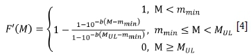
where

N_mmnis the number of events with magnitude greater than m_mn M_ULis the upper truncation magnitude of the distribution.

Similar to Equation [2], Equation [4] is a different formulation of a truncated and translated negative exponential distribution.

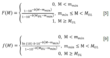
The cumulative distribution function, F(M) and the probability density functionJfM) for the TGR can be written as follows:

 

The M_maxconfusion

In the mining industry, the term 'M_max' is used for several different concepts, with the loose meaning of 'expected largest event' associated with it. These concepts are (see Figure 2):

 

 

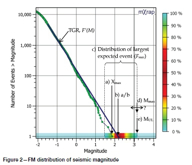
(a) the largest recorded event in a dataset (X_max)

(b) the value of the fitted GR relationship at N = 1 (a/b)

(c) the distribution of the largest expected magnitude (f_max)

(d) the largest physically possible event (M_max)

(e) the upper truncation of the FM distribution (M_UL).

Each of these is, in some way or another, being used as hazard indicators and they are discussed in the following paragraphs. Generally, no distinction is made between M_maxand M_UL, and the two concepts are mostly used interchangeably. Conceptually M_naahas a physical meaning, while M_ULcarries only the abstract meaning of being an upper limit of a probability distribution. I find it useful to keep these two concepts separated and will discuss this in more detail further on in the paper.

Due to the stochastic nature of seismicity, the largest event magnitude within a given number of events is a distribution and cannot be captured with a single number. This distribution is represented as a colour spectrum at N = 1 in Figure 2. In this paper, the probability density, cumulative probability and reverse cumulative probability functions of the distribution are respectively referred to as fmax, F_max, and F'_max.

It is important to note that any statement regarding the expectation of specified event magnitudes is dependent on the number of events. For any such statement to be meaningful, it is necessary to specify the number of events applicable to this statement. In this paper, the short notation, N@M, is used; for example, N@-1=100 or N@0 = 1, and the a-value in Equations [1] to [4] is equal to log(N@0).

 

Distribution of the expected largest event

The two parameters a/b and M_UL, shown in Figure 2 are important parameters in the assessment and communication of seismic hazard (Kijko and Funk, 1994; Jager and Ryder, 1999; Hudyma and Potvin, 2004; Hudyma, 2008; Mendecki, 2008; Hudyma and Potvin, 2010; Mendecki, 2012; Mendecki, 2013b). It appears though, that undue emphasis is sometimes placed on these parameters, which do not fully capture the seismic hazard. Consider the distribution of the maximum expected event within N@-1.5 = 4000, shown in Figure 2; the value of M_ULdefines only the upper limit of the F(M) and F_max(M) distributions and the a/b-value describes only one point on those distributions. The whole body of the distribution, however, describes the hazard.

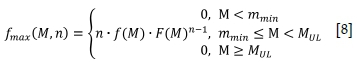
The distribution of the expected largest event can be obtained directly from the FM distribution. The cumulative distribution function of the largest magnitude within n events is given by (Gibowicz and Kijko, 1994):

where

F_max(M,n) is the cumulative distribution function of the magnitude of the largest event within n events

n is the the number of events with magnitude ≥ m_min

The probability density function of the largest event within n events can be obtained as the derivative of F_max and is as follows:

It is well-known that the intensity of dynamic waves attenuates sharply with distance. Using the Canadian Rockburst Handbook formulation (Mining Research Directorate, 1996), one can estimate that the body wave peak particle velocity (ppv) resulting from a Richter magnitude (M_L) of 3 at a distance of 500 m is similar to that from a M_L 0.5 at a distance of 20 m. Assuming a b-value of 1, one would expect about 315 events of ML > 0.5 for every single event of M_L > 3. When considering the fact that the workforce is exposed to the occurrence of many more small events at close proximity, it is clear that the body of the distribution, and not only the upper limit or the mode of the distribution, is important. This is evidenced in the fact that it is becoming more common to install face support in development headings to protect the workforce against the effect of events much smaller than the M_UL.

The consequence of smaller events is, of course, expected to be much smaller than that of an M_maxevent. One useful way to quantify the hazard, therefore, is to express it as the probability of exceeding a large event, for example, M_L1, M_L2, and M_L2.5 are commonly used, which for the illustration in Figure 2 are about 100%, 70%, and 30% respectively.

_{χ max}

By its very nature, the largest event in the data-set is a property of a data-set under consideration. For this reason, I prefer the convention employed by Gibowicz and Kijko (1994), and Kijko and Funk (1994), who refer to this value as X_max(the maximum value of set X) although M_obsor M°J¡X is also used in literature.

The value of X_maxis an indicator of hazard level in that it provides a lower bound of the largest event that can be expected in future Mm > X_max). Unless there is a significant and proven change in the conditions, the only defensible assumption is that an event larger than X_maxcan occur. This condition may be a significant change in the seismic regime that can be brought about by, for example, a change in the mining method or when mining moves from strong brittle ground into squeezing conditions.

X_maxis, of course, highly dependent on the size and representativeness of the subset of data under consideration and X_maxof the subset loses significance as a hazard indicator when a subset is temporally or spatially too small. X_maxas a hazard indicator captures only the historical experience and does not in any way account for the stochastic nature of seismicity.

 

THE a/b-value

The value of a fitted GR relationship at N = 1 is sometimes also referred to as 'a/b' (Hudyma, 2008) since it is equivalent to the ratio of the a and b parameters of the GR relationship (Equation [1]). It is important to note that a/b is a property of the fitted statistical model and not of the underlying data. The a/b-value is commonly used as an indicator of seismic hazard level with the meaning of 'the largest expected event' assigned to it.

It appears that this practice of interpreting a/b as the maximum event size is reinforced by the misunderstanding of the FM graph plotted for historical data (Figure 2). As the minimum value of the logarithmic y-axis is generally plotted as unity, and since no fractions of events can occur, this is interpreted as the 'end of the graph'. The GR relationship, however, is not a representation of the discrete events that occurred but a statistical best-fit model describing the relative frequency/probability of different sizes of event. There is no fundamental reason to stop the graph at N = 1. Interpreting the reverse cumulative distribution to terminate at N = 1 ignores the upper tail of the distribution, similar to the red line illustrated in Figure 3.

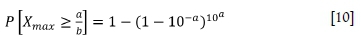
From the TGR distribution with the number of events determined by a, the probability of exceeding a/b is given by the following equation derived in Appendix A and plotted in Figure 4:

 

 

 

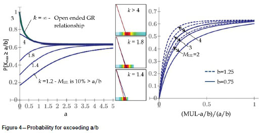
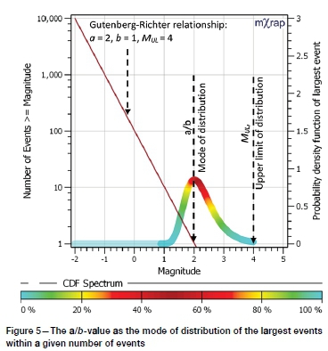
Which, for the open-ended GR relationship, reduces to the following:

where:

X_maxis the largest experienced event

b is the coefficient quantifying the log relative occurrence of smaller to larger events

a is the coefficient quantifying the number of events N@0 = 10^a

k is the Fraction by which M_ULis larger than a/b, i.e. M_UL= k · a/b

For an open-ended GR relationship, there is a > 63% chance of exceeding a/b. The probability is less for the truncated distribution. For situations where M_ULis large compared to a/b, the probability of exceeding a/b is large and the probability of exceeding a/b reduces for a/b closer to M_UL. The probability of exceeding a/b where a/b > M_ULis, per definition, zero. Note that these statements refer to the probability of exceeding a/b within the number of events determined by the a, i.e. N@0 = 10^a.

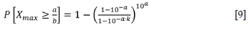
The a/b-value is an important parameter and it has a very clear meaning not generally appreciated. The a/b-value is the mode of the distribution of the largest event (the mode of fmax) (Figure 5). This is true for both the GR and TGR relationships (Appendix A).

 

 

The a/b-value is often used without consideration of spatial or temporal normalization, in which case it is a function of the subset of data under consideration and it loses any meaning as a hazard indicator. This will be discussed in greater detail further in he paper.

M_max and M_UL

[n physical terms, M_maxis used to define the region-characteristic maximum possible event magnitude, or, as the upper limit of event magnitude for a given region (Kijko and Singh, 2011). In other words, the largest magnitude that physical conditions will allow. In crustal seismology, this value is generally assumed to be constant for a particular seismic source zone. However, in the mining environment, the value of M_maxis not constant and is influenced by a number of factors, for example, rock mass conditions, mining-induced stress state, the mining sequence, and mining layout. In addition, M_maxis expected to increase with the extraction ratio (Mendecki, 2012).

As mentioned before M_maxand M_ra, are mostly used interchangeably. Conceptually M_maxhas the previously mentioned physical meaning, whilst M_ULcarries only the abstract meaning of being an upper limit of a probability distribution. I find it useful to keep these two concepts separate as one may choose to use a large value for M_UL, say M6, without implying that M_max= 6. The only implicit statement is that M_max< 6. Due to several difficulties which will be discussed in further detail in the following paragraphs, estimates of Mmax is subject to a great deal of uncertainty. For the purpose of hazard assessment and management, however, choosing a conservative but realistic value for M_ULwill suffice.

When assessing the probability of exceeding a specified magnitude P[M > M_f], underestimation of M_ULwith an error of δ (M_UL= M_max- δ) leads to larger errors than overestimation of M_UL by the same amount (M_UL= M_max+ δ). UnderestimatingM_ULis always optimistic, whilst overestimation is always conservative (Wesseloo, 2018). For the purpose of hazard assessment it is, therefore, prudent to use values for M_ULthat are deliberately conservative.

 

Estimating M_maxand M_UL

Wesseloo (2018) suggested the use of several methods discussed by Kijko (2004) to calculate M_maxplus the associated standard deviation, and assigning the maximum of these values to Μ_UL

where:

M_ULis a conservative but realistic upper limit for fmax.

M_{max t} is the largest magnitude that physical conditions will allow estimated with method i.

Δ_t is the standard deviation of the estimation of M_maxi

The reliable and robust estimate of M_max is not a trivial task and several researchers have invested considerable effort in finding reliable estimates from seismic event catalogues, with most of the effort directed at application in crustal seismology (e.g. Kijko and Funk, 1994; Kijko, 2004; Lasocki and Urban, 2011; Kijko, 2012). These methods, based on record statistics, aim to estimate the largest possible value based on the recorded data.

The simplest and most well-known method for estimation of M_ULis the Robson-Whitlock method formulated as follows (Kijko, 2004):

where

X_maxand X_max-1are the largest and second-largest recorded events

Among the other more common methods discussed by Kijko (2004) and (Kijko and Singh, 2011) are the Tate-Pisarenko, Kijko-Sellevoll, Order statistics, and Robson-Whitlock-Cooke and Cooke 1980.

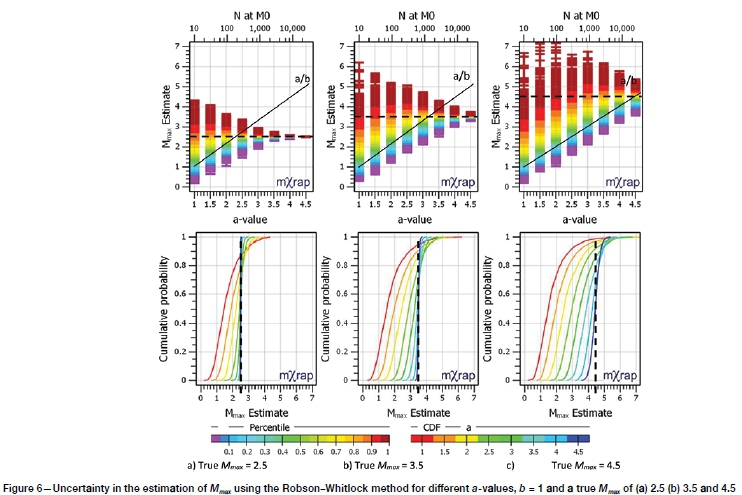
It is important to note that the reliability of the estimate of M_maxis highly dependent on the number of events on which this assessment is based. This dependence is investigated using Monte Carlo analysis on synthetically generated data-sets sampled from a specified FM distribution. For this analysis, M_max= 2.5, 3.5 and 4.5, b = 1, and a-values from 1 to 4.5 (N@0 = 10 to 32 000) were used. The results for the Robson-Whitlock method are shown in Figure 6. The value for M_maxis largely underestimated, with an underestimation of more 80% for an a/b < M_max- 1.

It is clear from the analysis that reasonably accurate estimates for M_maxcan only be obtained from large data-sets (N@0 > 1000 for M_max= 2.5 N@0 > 10 000 for M_max= 4.5). This implies that when the FM relationship is evaluated for smaller data-sets, the estimation M_maxshould not be limited to that small subset of data.

 

Artificial Black Swan events

 

The effect of variability

According to the Financial Times Lexicon, a Black Swan event is 'An event or occurrence that deviates beyond what is normally expected of a situation and that would be extremely difficult to predict.' Since the M_ULis the upper truncation of the FM distribution, any event with magnitude greater than M_UL is, per definition, assigned a zero probability of occurrence. Underestimation of M_UL, (M_UL < the true M_max), will assign a zero probability to magnitudes that could reasonably be expected, should the M_UL> the true value of M_max.

Consider the following example based on synthetic magnitude distribution data. Using random deviate sampling, magnitude values were sampled from a TGR relationship with the following properties: M_UL= 4, m_mln= -2, b = 1, and N@-2 is 100 000, i.e. a = 3. The results of several different approaches for estimating M_ULare shown in Figure 7.

Each of the sub-figures shows the FM distribution data; the best-fit GR (blue) and TGR (red) relationships. The probability distribution of the largest event for the given TGR relationship is shown as a spectrum at N = 1. The only differences between the sub-figures are the M_ULvalue and the resulting changes in the TGR relationship and the distribution of the largest eventsƒ_maxderived from it.

In Figure 7a, the value of M_UL= M_maxobtained with the Robson-Whitlock method (Equation [12]). In Figure 7b, M_ULis taken as the maximum of all of the methods listed in the previous section. In Figure 7c, the M_ULis taken as the maximum of all the aforementioned methods with an added standard deviation for each calculation, according to Kijko and Singh (2011), assuming a magnitude resolution of 0.1. Finally, in Figure 7d, M_UL= the true M_max= 4 is used. Even with M_UL calculated as the maximum of the mentioned methods (Figure 7b) or with Equation [11], the probability of M > 3.5 is zero and 12% respectively whilst the actual value is 20%.

The effect of sensor limitations

Apart from the underestimation of M_maxthat may occur simply due to variability in the data, underestimation may also result from limitations in the lower frequency limit of sensors. Morkel and Wesseloo (2017) described the problem occurring when the lower frequency limit of the sensors is not sufficiently low to record the low frequency content of large events and no correction for this effect is made. When this occurs, it will lead to the under-recording of the moment (and potency). Magnitude scales dependent on moment are thus susceptible to the underestimation of large magnitudes. This includes moment magnitude and magnitude scales defined as a function of both energy and magnitude. Since the estimation of energy is not sensitive to the under-recording of low frequencies (Boore, 1986), this effect is less pronounced for magnitude scales based on both energy and moment. Mendecki (2013a) performed a quick survey of 100 mines using IMS systems and found that 25% used a moment-based magnitude scale while the rest used a scale defined as a function of both energy and moment. For simplicity, the following discussion is limited to moment magnitude.

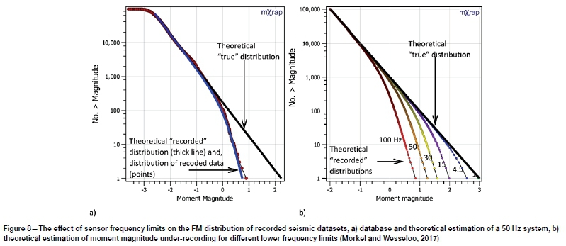
As a result of the under-recording of the low-frequency content and subsequent underestimation of the moment magnitude, the FM distribution of the recorded data exhibits a nonlinear (on the log-linear scale) relationship, as shown in Figure 8.

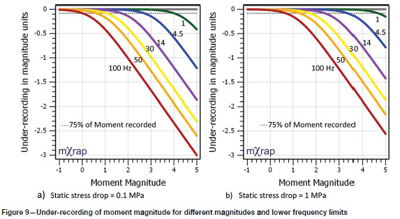
Figure 8a shows the FM distribution of recorded data from a mine network with only 50 Hz sensors. The downward curvature of the distribution is not a result of the underlying statistical behaviour of moment magnitude, but of the under-recording of the moment by the sensors. Also shown in the figure are two theoretical lines: the straight GR relationship assumed as the true distribution of moment magnitude; and a theoretical assessment of the effect of under-recording using analytical formulations (Boore, 1986; Di Bona and Rovelli, 1988; Mendecki, 2013a; Morkel and Wesseloo, 2017). The effect of different lower frequency limits of the sensors is illustrated in Figure 8b. The amount of under- recording for different moment magnitudes and lower frequency limits are shown in Figure 9.

 

 

For databases subjected to under-recording, underestimation of of M_maxwill result from the use of the statistical methods. To illustrate this problem, consider the following scenario plotted for N@0 = 300 in Figure 10. A seismic system with sensor lower limits of 14 Hz recording events from a seismic source with b = 1, M_maa= 3. Figure 10 shows the assumed FM distribution as a blue line, and the synthetic events sampled from that distribution as light grey. The dark blue points are adjusted for the frequency limit of the sensors, according to Boore (1986). The calculated value of M_max, in this case, is 2.53 which is smaller than the actual value of the largest experienced event on which the assessment is based, M2.68. The red line shows the truncated GR relationship based on the recorded events.

 

 

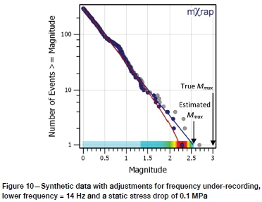
Similar responses also occur for other frequency limits but the magnitude range at which the deviation becomes significant, differs. The lower the frequency limit of the sensor, the larger the magnitude that will be adequately recorded.

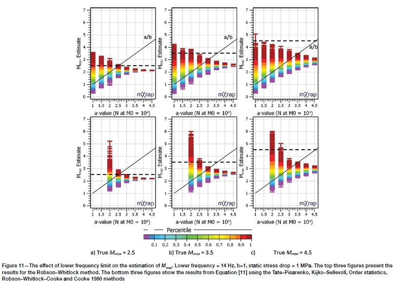
To further quantify the effect of the lower frequency of sensors on the estimation of M_max, a Monte Carlo analysis was performed, similar to that for which the results are shown in Figure 6. For this analysis, a lower frequency limit of 14 Hz and a static stress drop of 1 MPa are assumed. Excluding the added effect of the lower frequency of the sensor, these two analyses are the same. The results of this analysis are shown in Figure 11. The two sub-figures in column (a) display results for M_max= 2.5, (b) for M_max= 3.5, and (c) for M_max= 2.5. The top figure in each case presents the results for the Robson-Whitlock method. The results shown in the bottom figure in each case are obtained with Equation [11] using the Tate- Pisarenko, Kijko-Sellevoll, Order statistics, Robson-Whitlock-Cooke and Cooke 1980 methods.

It is clear from the comparison between Figure 6 and Figure 11 that the under-recording of moment due to sensor limitation can result in errors in the estimation of M_m(Wwhich are always optimistic and can be significant.

The best solution to this problem is to include lower frequency sensors in the system which are able to adequately record the lower frequency content of the event sizes expected at the mine (Figure 9). In lieu of this, corrections may be applied to the recorded values to compensate for the effect of the sensor under-recording (Morkel and Wesseloo, 2017).

 

Spatial distribution of seismic hazard

Probabilistic hazard calculation is commonly performed on data within spatial filters. Such spatial filters are often delineated with respect to mining infrastructure, often with arbitrary size. Such arbitrarily chosen volumes can have a significant influence on the assessment and may influence decision-making.

The sensitivity of hazard assessment to arbitrarily chosen volumes relates to the spatial distribution of b-value, the spatial distribution of events, and the difference in volume for these arbitrary spatial filters.

The influence of the spatial distribution of b-value

It is important to note that, when different seismic sources with different b-values are lumped together and the hazard calculated, the total hazard will be different from that when calculating the total hazard based on the separate sources.

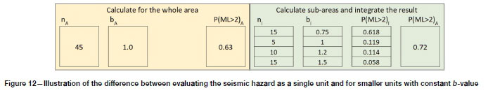
To illustrate this point, consider the idealized case illustrated in Figure 12 with a square subdivided into equal sub-areas on the left-hand side. On the right-hand side, the whole area is evaluated as a single unit. By way of analogy, these squares represent a mining area. For this illustration, we would like to answer the following question:

What is the probability ofM> 2 ?

For the purpose of this illustration, we will assume a constant event rate.

An approach often used in mining is to evaluate the whole area, A, (for example a large mining block or corridor) obtaining the a- and b-values for the whole area, and calculate the required probability value using the following equation.

where

m is a specified threshold magnitude

An alternative approach would be to calculate the a- and b-values for each of the sub-areas and calculate the overall probability as follows:

0The b-value for the combined area can be obtained from that of the sub-volumes as follows:

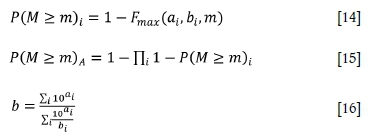
where:

a_i, b_i= a- and b-values for sub-volume i

It can be shown that for cases where the b-value over area A is constant, i.e. where b_t= b_A, the two approaches yield the same result. However, where this is not the case, the first approach does not yield the correct answer. For the example, in Figure 12 the difference between the two approaches leads to a difference of 9% probability of exceeding M2.

This illustration shows that the probabilistic evaluation representative of the volume under consideration can only be achieved by integration of the results obtained for each sub-volume where the sub-volumes are small enough to represent a volume with constant b-value.

The influence of the volume of spatial filters

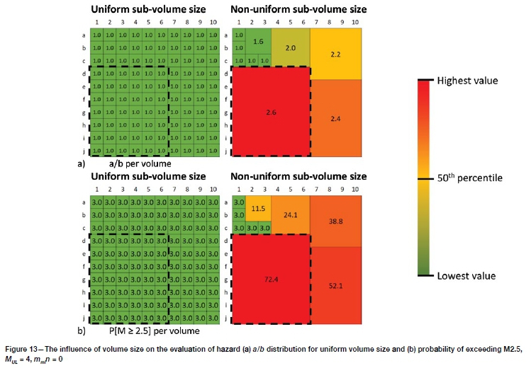
For a given b- and M_ULvalue, the number of events within a spatial filter will determine the seismic hazard for that spatial filter. The effect of hazard quantification and comparison between arbitrarily chosen spatial filter volumes without volume normalization is illustrated in Figure 13 and Figure 14. The square area shown on the left-hand side in Figure 13 and Figure 14 represents a whole mining area. In the left-hand side figures, the whole area consists of a hundred equally sized sub-areas which, for this example, each has a uniform distribution of events. The right-hand side figures display the same scenarios as that of the left-hand side figures, except that in these cases the whole mining area is subdivided into arbitrarily chosen spatial filter areas.

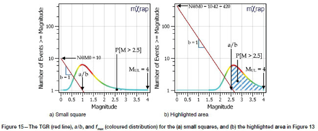
In Figure 13, the whole mine has the same seismic event rate of N@0 = 10 and b = 1. As a result, the spatial distribution of hazard is uniform throughout the whole mine with an a/b = 1 (Figure 13a left), and a probability of exceeding M2.5 at 3% per small square (Figure 13b left). The a/b-values and the probability of exceeding M2.5 are shown in the right-hand side figure for each of the arbitrary spatial filter volumes. The highlighted sub-area consists of 42 small areas and therefore has N@0 = 420. The TGR (red line), a/b,f_max(coloured distribution) for a small square and the highlighted area are shown in Figure 15.

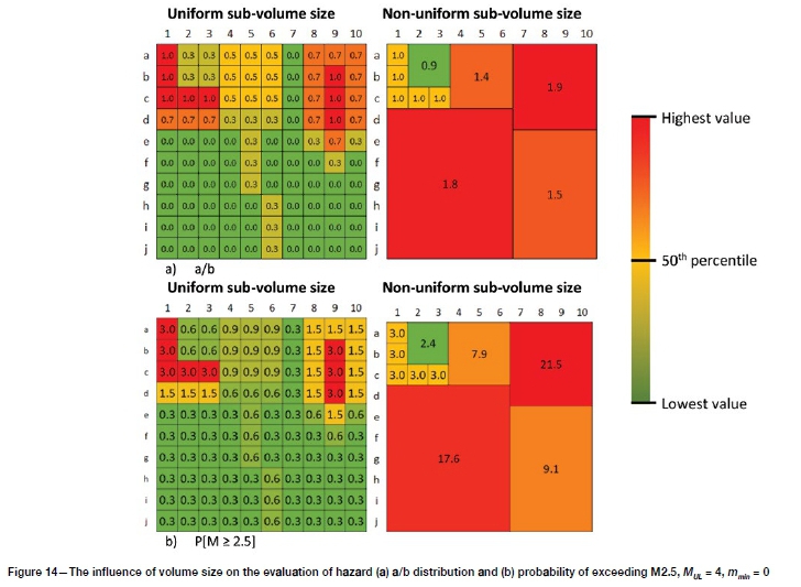
Evaluating the seismic hazard for arbitrary volumes leads to the amplification of the hazard for larger volumes and a misrepresentation of the hazard. Figure 14 illustrates the same effect in a different scenario where the event rate is not uniformly distributed throughout the whole mining area. Figure 14 illustrates the fact that arbitrarily chosen filter volumes can mask the true spatial distribution of seismic hazard. These comparative hazard maps can be corrected by normalizing the assessment with respect to the volume.

 

Hazard normalization

Spatial normalization

For the case illustrated in Figure 13, the statement was made that the probability of exceeding M2.5 per small square is 3%. In this statement, the hazard is normalized with respect to volume. This normalized value is essential for obtaining a spatial distribution of hazard or a true comparison of hazard between different volumes but it does not provide the absolute hazard. The hazard for the whole mining area is not 3%. For the whole mining area, we need to integrate the hazard of each of the sub-areas to obtain 95%. In other words, there is about a 95% chance of experiencing M2.5 anywhere in the mine, but it is equally likely to occur anywhere in the mine with a 3% probability of occurring in any one of the small squares.

The total hazard for the whole mine and the spatial distribution of that hazard are independent of the size of the small squares, but the actual value associated with the small square is dependent on the size of the squares. To represent the spatial distribution in a way that is independent of the sub-square size, one would need to define a characteristic volume to which all values are normalized. It should be noted that the size of a characteristic volume does not influence the hazard calculations nor the spatial hazard distribution, but only influences the actual numbers by which the hazard is expressed. Wesseloo (2018) suggested the use of a volume size equal to that of a sphere with a radius of 50 m. The a/b-values in the scenario shown in Figure 14 are spatially normalized to a characteristic volume shown in Figure 16a.

 

 

The sub-square size of 20 m was assumed, and since the example is a two-dimensional one, an equivalent representative area with radius 50 m was used. The comparison between the non-uniform sub-volume scenarios in Figure 14a and Figure 16a shows that the normalization to a characteristic volume enables a more reasonable comparison of seismic hazard distribution. Spatial normalization, however, does not correct for the loss of information that occurs when the spatial filters do not take account of the underlying seismic sources, as only a mean value for each sub-volume is retained. As a result, some masking of seismic hazard trends still occur. The left-hand side diagram of Figure 16a illustrates the fact that when the evaluation volume is small enough to capture the change in seismic sources in space, the normalized a/b values provide a useful hazard rating for quantifying the spatial distribution of the seismic hazard.

Wesseloo (2018) takes this one step further and defines a hazard rating based on the same definition for the characteristic volume. The hazard rating is defined as the magnitude with a 15% probability of exceedance within the equivalent representative volume. This hazard rating definition was chosen to produces similar rating values to the hazard scale originally proposed by Hudyma and Potvin (2004), with which many mines in Australia and Canada are familiar. For the scenario in Figure 14b, this leads to the spatial hazard rating shown in Figure 16b. This approach provides a method for representing the spatial distribution of hazard which is independent of the size of the sub-volume.

Time normalization

The normalization of hazard is as important in the time domain

as it is in space. To enable direct comparison between hazards of different durations, it is necessary to normalize the calculated probability to the same equivalent timescale. This normalization can be performed as follows (Wesseloo, 2018):

where

Tn, Te are the normalized timeframe and the original timeframe, respectively

P_Tn, P_Teare the equivalent probabilities expressed for timeframes Tn and Te, respectively

A hazard with a weekly probability of 1% can be expressed with equivalent annualized values as 1 - (1 - 0.01)⁵² = 40%, while a hazard with a biennial probability of 50% can be expressed in equivalent annualized values as 1 - (1 - 0.5)⁰ = 30%.

Normalization can be performed to any timescale but short time periods should be avoided as this leads to small numbers which are often misinterpreted as small hazards. The use of one year (annualization) seems a reasonable approach and corresponds with the practice in other branches of engineering, financial risk management and corporate governance (Jonkman, van Gelder, and Vrijling, 2003; Terbrugge etal., 2006; Stacey, Terbrugge, and Wesseloo, 2007; Wesseloo and Read, 2009). Annualization also allows one to calculate the associated risk and evaluate it against corporate accepted annualized risk levels.

Annualization of hazard values leads to an 'annual probability', but it is important to note that this should not be interpreted as the probability for a physical year (future or historical). It is the probability value appropriate to the timescale for which the mean seismic rate is applicable, expressed in equivalent annualized terms.

The example calculations following Equation [17] assume that both hazards are present over a long time period. If, for example, a hazard with a weekly probability of 1% is present only for one week in the year, the yearly hazard would also be 1%. This sometimes leads to misunderstanding in the application of hazard assessments in industry where a short-lived but repeating hazard is sometimes evaluated in isolation.

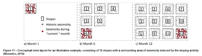
Seismic hazard in a mine is transient in space and time and, although the seismic hazard at a specific location might be short-lived, the hazard is of a repeating nature. For example, the hazard associated with the mining of a single stope might be present only during the time it takes to mine that stope, but, a similar hazard might occur due to the mining of the next stope. Both long-term and repeating hazards can be normalized temporally using Equation [17].

Wesseloo (2018) illustrated this concept with the following fictitious mining scenario that consists of 12 stopes (Figure 17). Each of the stopes is mined for a month, during which a seismic response is induced in the indicated area around it. The seismicity in this surrounding area ceases when mining in this stope is complete. During the following month, the next stope is mined with the associated induced seismicity limited to its surrounding area. The argument can be further simplified by assuming a constant b = 1 over the whole volume and the whole year, and by assuming that the total number of events occurring in the surrounding area of each of the stopes is the same at N@-2 = 1000 (a = 1).

For each stope, the probability of exceeding M2 is 3.92%, and if evaluated in isolation, may be regarded as acceptable. Cumulating the number of events for all 12 stopes, however, results in the total probability of exceeding M2 of 38%. In the year, the company is exposed to the total aggregated hazard of P[M > 2] = 38%, even though each stope only has an individual monthly hazard of probability 3.9%. If exposing the company to the yearly hazard of 38% is not acceptable, by implication, it is not acceptable to expose the company to the hazard associated with every one of those stopes individually.

 

Conclusing remarks

The topic of seismic hazard assessment is subject to several misconceptions in the mining industry, and this paper addressed some of these. The term 'M_maX is used for several different concepts which appear to contribute to these misconceptions. To avoid confusion, I suggest that the term 'M_max' should be reserved for the concept of the maximum credible event. Other concepts referred to as 'M_max' should be referred to by unique names. I propose the use of 'X_max' or 'M_obs' for the largest recorded event in a data-set, 'a/b for the value of the fitted GR relationship at N = 1, and, 'M_UL' for the upper truncation value of the FM distribution.

The value of the fitted GR relationship at N = 1 (a/b) is sometimes interpreted as the expected largest event. This value is, however, the mode of the distribution of the largest expected magnitude with a 63% chance of being exceeded for the open-ended GR relationship. The probability of exceedance is smaller for truncated GR relationship and depends on the upper limit of the distribution.

The accuracy of methods for estimating M_maxis low when a/b << M_maxand tends to underestimate M_max. Reliable results can only be obtained when M_maxis based on large data-sets, (e.g. N@0 > 1000 for M_maa= 2.5 N@M > 10 000 for M_maa= 4.5).

When assessing the probability of exceeding a specified magnitude P[M > M_t], underestimation of (M_UL= M_max- δ) leads to larger errors than overestimation of M_ULby the same amount (M_UL = M_max+ δ). Underestimating M_ULis always optimistic, while overestimation s always conservative. For the purpose of hazard assessment, it is therefore prudent to use values for M_ULthat are deliberately conservative.

Artificial Black Swan events can be created when M_UL underestimates M_max. This can occur simply due to the effect of uncertainty. The under-recording of low frequencies due to sensor limitations leads to the underestimation of M_maxand also leads to artificial Black Swan events. To combat this problem, sensors which are able to adequately record the lower frequency content of the event sizes expected at the mine, need to be included in the system. In lieu of this, corrections may be applied to the recorded values to compensate for the effect of the sensors under-recording.

Assessment of the seismic hazard needs to be performed on sub-volumes for which the b-value and the event rate can be assumed to be constant.

For comparative hazard evaluation in space and time, both spatial and temporal normalization are necessary. Normalization to a characteristic volume equal to a sphere with a 50 m radius is suggested. Annualization of hazards is proposed for temporal normalization.

 

Acknowledgements

I thank William Joughin and Lindsay Linzer for their valuable comments on the manuscript. I also thank all my colleagues at the ACG for their support and, in particular, Yves Potvin, Gerhard Morkel, Kyle Woodward, Dan Cumming-Potvin and Stuart Tierney for fruitful technical discussions. I also would like to thank Paul Harris and Matt Heinsen Egan for always being available to help me with any scripting troubleshooting and app building in mXrap. Thanks also to Josephine Ruddle and Christine Neskudla for proofing my language. The content of this paper has flowed from work done over the span of several years with the support of the mXrap Consortium.

 

References

Boore, D. 1986. The effect of finite bandwidth on seismic scaling relationships. In earthquake source mechanics.         [ Links ]

Das, S., Boatwright, J. and Scholz, C.H. (eds.), American Geophysical Union, Washington, pp. 275-283.         [ Links ]

Di Bona, M. and Rovelli, A. 1988. Effects of the bandwidth limitation of stress drops estimated from integrals of the ground motion. Bulletin of the Seismological Society of America, vol. 78, no. 5. pp. 1818-1825.         [ Links ]

Financial Times. Financial times lexicon http://lexicon.ft.com/ [Accessed 22 March 2019].         [ Links ]

Gibowicz, S.J. and Kijko, A. 1994. An introduction to mining seismology. Academic Press, San Diego.         [ Links ]

Gutenberg, B. and Richter, C.F. 1944. Frequency of earthquakes in California. Bulletin of the Seismological Society of America, vol. 34, no. 4. pp. 185-188.         [ Links ]

Hudyma, M. and Potvin, Y. 2004. Seismic hazard in Western Australian mines. Journal of The South African Institute of Mining and Metallurgy, vol. 104, no. 5. pp. 265-275.         [ Links ]

Hudyma, M. and Potvin, Y.H. 2010. An engineering approach to seismic risk management in hardrock mines. Rock Mechanics and Rock Engineering, vol. 43, no. 6. pp. 891-906.         [ Links ]

Hudyma, M.R. 2008. Analysis and interpretation of clusters of seismic events in mines. PhD thesis, University of Western Australia.         [ Links ]

Jager, A.J. and Ryder, J.A. 1999. A Handbook on Rock Engineering Practice for Tabular Hard Rock Mines. Safety in Mines Research Advisory Committee (SIMRAC), Johannesburg.         [ Links ]

Jonkman, S.N., van Gelder, P.H.A.J.M., and Vrijling, J.K. 2003. An overview of quantitative risk measures for loss of life and economic damage. Journal of Hazardous Materials, vol. 99, no. 1. pp. 1-30.         [ Links ]

Kijko, A. 2004. Estimation of the maximum earthquake magnitude, mmax. Pure and Applied Geophysics, vol. 161, no. 8. pp. 1655-1681.         [ Links ]

Kijko, A. 2012. On Bayesian procedure for maximum earthquake magnitude estimation. Research in Geophysics, vol. 2, no. 1. pp. 46-51.         [ Links ]

Kijko, A. and Funk, C. 1994. The assessment of seismic hazards in mines. Journal of the South African Institute of Mining and Metallurgy, vol. 94, no. 4. pp. 179-185.         [ Links ]

Kijko, A. and Singh, M. 2011. Statistical tools for maximum possible earthquake magnitude estimation. Acta Geophysica, vol. 59, no. 4. pp. 674-700.         [ Links ]

Lasocki, S. and Urban, P. 2011. Bias, variance and computational properties of Kijko's estimators of the upper limit of magnitude distribution, Mmax. Acta Geophysica, vol. 59, no. 4. pp. 659-673.         [ Links ]

Mendecki, A.J. 2008. Forecasting seismic hazard in mines. Proceedings of the First Southern Hemisphere International Rock Mechanics Symposium, SHIRMS 2008. Potvin, Y., Carter, J., Dyskin, A. and Jeffrey, R. (eds.). Australian Centre for Geomechanics, Perth, Western Australia. pp. 55-69.         [ Links ]

Mendecki, A.J. 2012. Keynote lecture: Size distribution of seismic events in mines. Proceedings of the Australian Earthquake Engineering Society Conference. Australian Earthquake Engineering Society, pp. 20.         [ Links ]

Mendecki, A.J. 2013a. Frequency range, Log E, Log P and magnitude. Proceedings of the Eighth International Symposium on Rockbursts and Seismicity in Mines - RaSiM8. Malovichko, A. and Malovichko, D., (eds.). Geophysical Survey of Russian Academy of Sciences, Mining Institute of Ural Branch of Russian Academy of Sciences. pp. 167-180.         [ Links ]

Mendecki, A.J. 2013b. Keynote lecture: Characteristics of seismic hazard in mines. Proceedings of the Eighth International Symposium on Rockbursts and Seismicity in Mines, RaSiM8. Malovichko, A. and Malovichko, D., (eds.). Geophysical Survey of Russian Academy of Sciences, Mining Institute of Ural Branch of Russian Academy of Sciences. pp. 275-292.         [ Links ]

Mining Research Directorate. 1996. Canadian rockburst research program 19901995, a comprehensive summary of five years of collaborative research on rockbursting in hardrock mines. CAMIRO Mining Division, Sudbury, Ontario.         [ Links ]

Morkel, I.G. and Wesseloo, J. 2017. The effect of sensor bandwidth limitations on the calculation of seismic hazard for mines. Proceedings of the Ninth International Symposium on Rocbursts and Seismicity in Mines. Vallejos, J.A., (ed.), Ediarte S.A., Envigado, Columbia. pp. 42-49.         [ Links ]

Page, R. 1968. Aftershocks and microaftershocks of the great Alaska earthquake of 1964. Bulletin of the SeismologicalSociety of America, vol. 58, no. 3. pp. 1131-1168.         [ Links ]

Potvin, Y., Wesseloo, J., Morkel, G., Tierney, S., Woodward, K., and Cuello, D. 2019. Seismic risk management practices in metalliferous mines. Proceedings of the Ninth International Conference on Deep and High Stress Mining. Joughin, W.C., (ed.). Southern Africa Institute of Mining and Metallurgy, Johannesburg. pp. 123-132.         [ Links ]

Stacey, T.R., Terbrugge, P.J., and Wesseloo, J. 2007. Risk as a rock engineering design criterion. Challenges in Deep and High Stress Mining. Potvin, Y., Stacey, T.R., and Hadjigeorgiou, J. (eds.), Australia, Australian Centre for Geomechanics, Perth. pp. 19-25.         [ Links ]

Terbrugge, P.J., Wesseloo, J., Venter, J., and Steffen, o.K.H. 2006. A risk consequence approach to open pit slope design. Journal of the South African Institute of Mining and Metallurgy, vol. 106, no. 7. pp. 503-511.         [ Links ]

Utsu, T. 1999. Representation and analysis of the earthquake size distribution: A historical review and some new approaches. Pure and Applied Geophysics, vol. 155, no. 2-4. pp. 509-535.         [ Links ]

Wesseloo, J. 2018. The spatial assessment of the current seismic hazard state for hard rock underground mines. Rock Mechanics and Rock Engineering, vol. 51, no. 6. pp. 1839-1862.         [ Links ]

Wesseloo, J. and Read, J. 2009. Acceptance criteria. Guidelinesfor Open Pit Slope Design. Stacey, P. and Read, J. (eds.). CSIRO Publishing, Australia. pp. 221-236.         [ Links ]

 

 

Correspondence:
J. Wesseloo
johan.wesseloo@uwa.edu.au

Received: 29 Jun. 2019
Revised: 5 Dec. 2019
Accepted: 11 Dec. 2019
Published: January 2020

 

 

1 Also referred to as Complementary Cumulative Distribution or Inverse Cumulative Distribution. The term 'Inverse Cumulative Distribution', however, is also used to refer to the quantile function.

 

 

Appendix A

The probability of exceeding an event size of a/b within n events

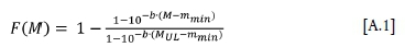
For the TGR relationship, the CDF of the event distribution from the magnitude of completeness m_minis then given by

The probability of exceeding an event size of M within n events is given by (Gibowicz and Kijko, 1994):

where:

F_max(M) is the cumulative distribution function of the magnitude of the largest event

F(M) is the cumulative probability density function describing the magnitude distribution of event size.

The probability of exceeding the value of a/b within n events of magnitude > mmin is given by

And defining M_UL= k-a/b leads to

This relationship is independent of m_minand can be written in terms of the a-value as

which, for the open-ended GR relationship reduces to

The mode of the distribution of F_max

The mode of f_max(x) can be obtained as follows:

which reduces to x = a/b for both the open-ended and TGR relationship. ♦