GENERAL PAPERS

 

Weibull failure analysis of seismic event return periods in the Far West Rand and Klerksdorp-Orkney-Stilfontein-Hartebeesfontein gold mine areas

 

 

M.B.C. Brandt

Council for Geoscience, Engineering and Geohazards Unit, South Africa

Correspondence

 

 

---

SYNOPSIS

Weibull failure analyses of seismic event return periods in the Far West Rand (FWR) and Klerksdorp-Orkney-Stilfontein-Hartebeesfontein (KOSH) gold mine areas were completed for the period October 2012 to January 2018. The analyses reveal that seismic event occurrences in the gold mines mostly follow a Poisson process for magnitudes M > 2. This implies that the event catalogue for a classical hazard analysis does not require declustering, provided mining activities and the time-of-day pattern are constant throughout the period. The Weibull analyses were benchmarked against event occurrences in the southern California earthquake catalogue. Two failure systems for small and larger events with short and longer return periods, respectively, were identified. An excessive number of dependent events with short return periods were interpreted as fore- and aftershocks. The FWR and KOSH sub-catalogues reveal comparable, but also different, event occurrences to those for southern California. Very few dependent events could be recognized for short return periods, rather than the excessive number of events expected when assuming a Poisson process. Two failure systems were identified for lower-magnitude events with longer return periods. For KOSH, the two failure systems were found to overlap at lower magnitudes than for FWR.

Keywords: Weibull analysis, mining-related seismic event, return period.

---

 

 

Introduction

In classical seismic hazard analysis applied in many South African gold mines, the parameters that describe the hazard are the seismic activity rate, X, the Gutenberg-Richter value, b and, occasionally, the maximum regional magnitude, m_max. The activity rate may be calculated by its definition, λ = n/T, where n is the total number of events with magnitudes greater than or equal to the completeness threshold and T denotes the time span of the event catalogue. The mean return period (mean time interval) between seismic events having a magnitude equal to or greater than m is given by Rp(m) = 1/λ(m). In hazard analysis, the sometimes unspoken assumption is that the occurrence of seismic events in time follows a Poisson process (Kijko and Funk, 1994). A Poisson process has waiting times between events that are independent, identically distributed, and memoryless. Hence, the occurrence of a new event is independent of previous events, as in radioactive decay (e.g. Feller, 1971). However, this does not seem to be the case for the Far West Rand (FWR) and Klerksdorp-Orkney-Stilfontein-Hartebeesfontein (KOSH) gold mines. A daily seismicity pattern is identifiable in the time-of-day distribution recorded by the South African National Seismograph Network for events in 2006 (Saunders et al., 2011) which could indicate the presence of a significant number of dependent events in the earthquake catalogue. On the other hand the inter-event time distribution of larger seismic events in most of the mines is random, even though over the short term small seismic events tend to occur in clusters in space and time in response to rock extraction (du Toit and Mendecki, 2007). These processes are neither stationary nor independent. However, if a number of such processes are superimposed over a longer time and a larger area the outcome is thought to become random (du Toit and Mendecki, 2007). It is hence uncertain whether a seismic hazard analysis is valid if a Poisson process in time is assumed for larger seismic event occurrences of magnitude M > 2.

A mostly Poisson process for tectonic earthquake occurrence is assured in classical hazard analyses by first 'declustering' the catalogue. This involves the removal of fore- and aftershocks (or, alternatively, of dependent events) leaving only main shocks (or independent events) for the analysis (e.g. Luen and Stark, 2012). A similar approach may be followed for a South African mine catalogue. A time-of-day filter that excludes events during blasting time may be applied to remove dependent events from the catalogue, leaving behind only main shocks. However, the entity 'main shock' in this residual catalogue is not clear for mine-related seismicity. It is uncertain whether rejected dependent events have smaller magnitudes than the 'main shocks', as is the case for tectonic aftershocks that follow Omori's Law (Omori, 1895). Removing dependent events appears to be inappropriate since the exclusion of potentially damaging events from the catalogue may lead to a flawed seismic hazard analysis.

The goal of this study is to ascertain whether seismic event occurrences in the gold mines indeed follow a mostly Poisson process in spite of the daily patterns, i.e. to establish whether a classical hazard analysis requires declustering. This will be accomplished by applying a Weibull failure analysis on the return periods of the discrete magnitudes, from magnitudes greater than or equal to the completeness threshold up to the largest magnitude with a sufficient number of observations. Weibull failure analyses are often applied in industry to estimate the failure rate of components or other phenomena. The Weibull distribution is, in simple terms, an expanded exponential distribution which allows for the classification of failures over time as a Poisson, or other, process (e.g. Abernethy, 2004; Lai, Pra Murthy, and Xie, 2006). The analysis method will first be tested on a tectonic earthquake catalogue from California which is expected to contain readily identifiable fore- and aftershocks. This will be followed by analyses of the event catalogues for the FWR and KOSH. The results of the FWR and KOSH analyses will be compared with one another and benchmarked against those from the southern California analysis.

 

Weibull failure analysis

The Weibull distribution is one of the best-known lifetime distributions. It describes observed failures of many different types of components and phenomena (e.g. Lai, Pra Murthy, and Xie, 2006). Weibull failure analysis is widely used today, for example, in the aeronautic and automotive industries, to evaluate the reliability of products, to carry out failure forecasts, for engineering change test substantiation, maintenance planning, and system performance analysis (e.g. Abernethy, 2004). The distribution was introduced by Waloddi Weibull, who first used the methodology to model the breaking strength of materials (Weibull, 1939) and later for a wide range of other applications (Weibull, 1951). The commonly used two-parameter Weibull cumulative distribution function (CDF) is (e.g. Abernethy, 2004):

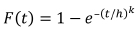
where t is the failure time, k is the shape parameter, h is the scale parameter (also known as the characteristic life), and e is the base for the natural logarithm. The corresponding probability density function (PDF) is:

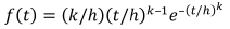
The shape parameter, k, determines the class of failure mode, as shown in Figure 1. Parameter h mostly scales the time axis. Four failure classes may be identified for constant h.

 

 

> A value of k < 1 indicates that the failure rate decreases over time. This happens if there is significant 'infant mortality' or 'teething problems', or where defective items fail early with a failure rate decreasing over time as the defective items are weeded out of the population. This distribution is fat-tailed and in earthquake seismology is known as the stretched exponential distribution.

> A value of k = 1 indicates that the failure rate is constant over time. This may suggest that random external magnitudes than the 'main shocks', as is the case for tectonic aftershocks that follow Omori's Law (Omori, 1895). Removing dependent events appears to be inappropriate since the exclusion of potentially damaging events from the catalogue may lead to a flawed seismic hazard analysis.

x> A value of k > 1 indicates that the failure rate increases with time. This happens if there is an 'ageing' process, for example, if parts are more likely to wear out and/or fail over time. This distribution is thin-tailed.

> A value of k > 4 indicates that the failure rate rapidly increases with time. This happens if 'old age' sets in, for example, where the entire fleet/system fails as it reaches the end of its life-span.

The physics of the system, the type of problem, the available observations, and the purpose of the analysis determine how the Weibull analysis is set up. To illustrate Weibull analysis with an example: in the case of a specific type of jet engine, the failure time may be defined as the time that has lapsed since its manufacturing or installation. Alternatively, only the time during which the engine was in use, or the time that has lapsed since the last service, may be taken into consideration. Failure may be classified as normal wear and tear, a minor fault, a major failure, or catastrophe. Since a jet engine comprises many components the Weibull analysis may reveal a mixture of failure modes as different parts fail in several ways (Figure 1). A minor fault of one component may also lead to a major failure of another, dependent part, or vice versa, where a major failure causes multiple minor faults (e.g. Abernethy, 2004; Lai, Pra Murthy, and Xie, 2006).

The Weibull failure analysis of seismic events will be performed using the CumFreq software (Oosterbaan, 2018). Failure time per magnitude class is defined as the time that has lapsed since the previous failure - known in seismology as the return period (time interval). The CumFreq calculator models the cumulative frequency distribution and fits it to a probability distribution. The software can accommodate 20 different probability distributions, including exponential and Weibull distributions. The analysis steps are as follows:

> Select a number of equal intervals of widths suited to the data series and the purpose of the analysis.

> Count the number of data-points in each interval. The number in each interval is divided by the total number of data-points to obtain the frequency of data-points for each interval.

> The data for frequency analysis is ranked in descending order, with the highest value first and the lowest last. For an earthquake catalogue, the latter is trivial since events with smaller magnitudes usually occur more frequently than larger ones.

> Calculate the cumulative frequency as the sum of the frequencies over the intervals below a chosen limit. Note that, by definition, the sum of the frequencies over all intervals equals unity.

> Estimate the parameters of the cumulative frequency distribution (e.g. k and h of the Weibull CDF) by means of a linear regression. Where k = 1, this simplifies to the exponential CDF and a second pass with an exponential distribution usually yields more stable results.

> The 90% upper and lower confidence limits are calculated last (Oosterbaan, 1994).

 

Analysis of southern California seismic event return periods

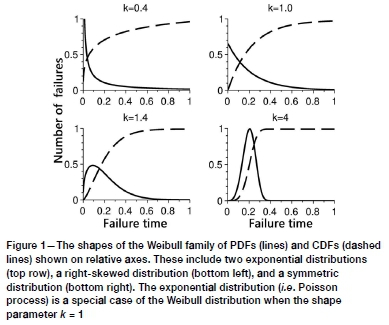
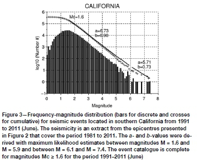
For the benchmark Weibull analysis, the relocated catalogue for southern California from 1981 to June 2011 (Hauksson, Yang, and Shearer, 2012) was downloaded from the Southern California Earthquake Center. The epicentres are presented in Figure 2. To derive this catalogue, the authors combined double difference locations obtained by means of hypoDD (Waldhauser and Ellsworth, 2000) with those determined using 3D velocity models (Thurber, 1993). This yielded a complete catalogue with improved clustering of hypocentres. Quarry blasts and other anthropogenic events were removed and unstable hypocentres deeper than 30 km were rejected. The authors recommend using the catalogue for the interpretation of spatial and temporal seismicity patterns. The catalogue with its event clustering is expected to contain readily identifiable fore- and aftershocks suitable for a Weibull analysis in view of classifying earthquakes over time as following a Poisson or other process. The frequency-magnitude distribution, shown in Figure 3, reveals two populations of events with different b-values that change between M = 5.9 and M = 6.1.

 

 

 

 

Events in three representative sub-catalogues with magnitudes M = 3.1, 4.2, and 5.2 with bin size M = 3.1 ± 0.05, 4.2 ± 0.05, and 5.2 ± 0.05 were selected for the analysis. An insufficient number of events with magnitudes M > 5.2 had been observed for conclusive analyses. The Weibull CDF parameters, k and h, were first determined with an unrestricted linear regression. For magnitudes M = 3.1 (Figure 4) and M = 4.2 the CumFreq calculator rejected the first interval observation (the very short return periods with an excessive number of events) and derived a value for k = 1.10229 and k - 1, respectively. Given the qualitative shape of the observations in relation to Figure 1, further regressions were restricted to 0.1 < k < 0.5. These calculated CDFs failed to fit the observations, as most of the observations plotted outside the 90% confidence limit. A second pass with an exponential CDF yielded good fits for both of the above sub-catalogues (excluding very short return periods), as is evident from Figure 5. For magnitude M = 5.2 there were no excessive events for very short return periods and the unrestricted regression again yielded the result k => 1. Hence the final result was also derived for an exponential CDF. Note that the exponential parameter, a = 1/h, decreases with increasing magnitudes as the return periods become longer.

All the observed interval frequencies of the event return periods for M = 3.1 plotted above the calculated interval frequencies in Figure 5. This violates the requirement that the sum of the calculated frequencies over all intervals must equal unity. It indicates that even though many of the observations plotted inside the 90% confidence limit the fit may be improved with an unrestricted linear regression. Observed interval frequencies plotted above and below the calculated interval frequencies and observations better fitted the 90% confidence limit in Figure 4. For magnitudes M = 4.2 and M = 5.2, observed interval frequencies plotted above and below the calculated interval frequencies for the exponential CDFs in Figure 5. An unrestricted linear regression improved these fits only marginally. The derived shape parameter, k, of 1.10229 for M = 3.1 was close enough to k = 1 to accept the result of the exponential CDF as an adequate fit.

The qualitative patterns are illustrated in Figure 5:

> For small magnitudes (M = 3.1), the observed interval frequencies of event return periods decrease monotonically from short to longer, with an excessive number of very short return periods. No event with a return period of more than 25 days is observed.

> For larger magnitudes (M = 4.2), the observed interval frequencies decrease monotonically from short to a longer 45 days, with an excessive number of very short return periods. A significant number of events have return periods of more than 45 days - these were excluded from the Weibull analysis.

> For large magnitudes (M = 5.2), the observed interval frequency decreases monotonically from fairly short to a much longer 2825 days. The excessive number of very short return period events has disappeared and only one event has a return period of less than 45 days.

Two failure systems with dependent, smaller events may be identified from the PDF and CDF in Figure 5.

> The first failure system includes event occurrences that follow a Poisson process for small (approx. M = 3.1) to larger (approx. M = 4.2) magnitudes, with return periods up to 45 days. For larger events, a second failure system emerges with longer return periods beyond 45 days.

> An excessive number of events are observed for small (approx. M = 3.1) to larger (approx. M = 4.2) magnitudes with very short return periods. These event occurrences do not follow a Poisson process but cannot be classified as 'infant mortality' or 'teething problems' that may have indicated weak areas in the fault zones with numerous 'failures'. These events are thought to be fore- and aftershocks that are dependent on larger-magnitude events and, hence, could follow Omori's Law (1895). These events may be those that are removed from a catalogue as a result of 'declustering' before performing a seismic hazard analysis.

> The second failure system includes event occurrences that follow a Poisson process for large (approx. M = 5.2 magnitudes with fairly short to very long return periods. The two failure systems overlap for larger (approx. M = 4.2) magnitudes.

 

Analysis of Far West Rand and Klerksdorp-Orkney-Stilfontein-Hartebeesfontein seismic event return periods

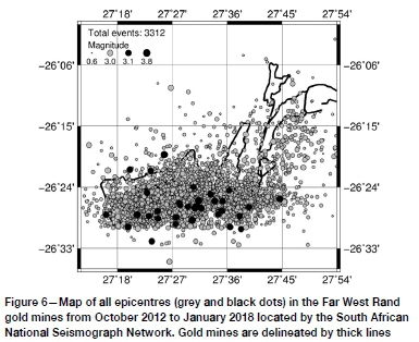
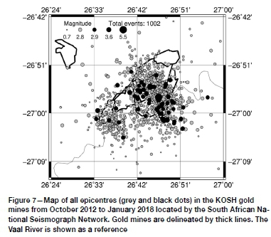
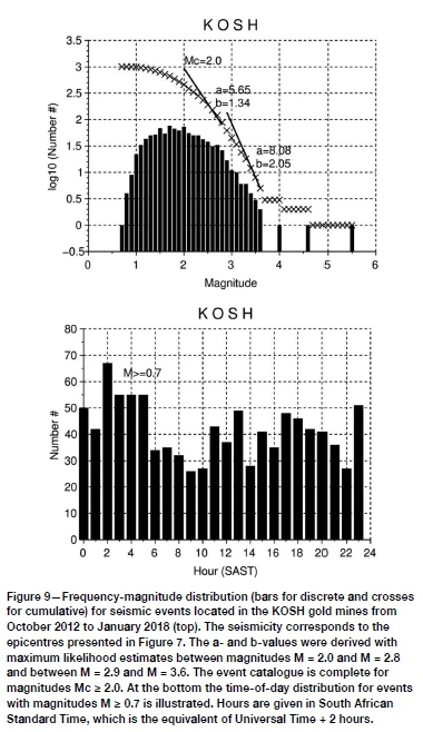
The FWR and KOSH catalogues were obtained from epicentres routinely located by the South African National Seismograph Network from October 2012 to January 2018 (Saunders et al., 2008) for which time period a calibrated local magnitude scale had been implemented (Saunders et al., 2012). Epicentres are presented for the FWR and KOSH in Figures 6 and 7, respectively. Seismicity patterns in the frequency-magnitude and time-of-day distributions are illustrated in Figures 8 and 9. The FWR frequency-magnitude distribution revealed two populations of events with different b-values and a daily seismicity pattern with a peak in the afternoon. No daily pattern could be identified for KOSH. The frequency-magnitude distribution also identified two populations for KOSH with b-values that change between M = 2.8 and M = 2.9. The two largest events observed in the FWR had magnitudes of M = 3.8 and the three largest (characteristic) events observed in the KOSH had magnitudes of M = 4.0, M = 4.6, and M = 5.5.

 

 

 

 

 

 

 

 

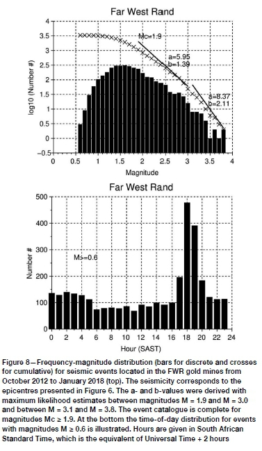
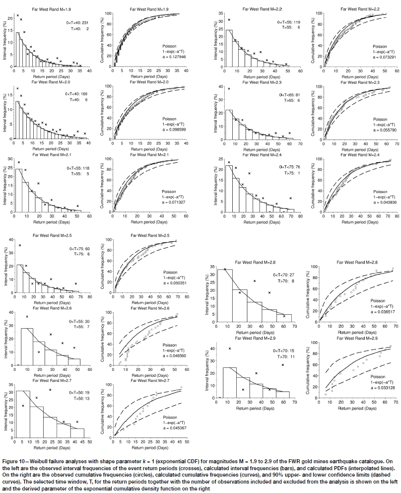
Weibull analyses for the FWR were performed using events from a completeness magnitude of M = 1.9 (Brandt, 2019) up to magnitude M = 2.9, for which a sufficient number of events had been observed. This excluded mine blasts, which are thought to have magnitudes smaller than M = 1.9. The FWR sub-catalogues reveal comparable, but also different, qualitative patterns to those for southern California and are illustrated in Figure 10.

> For small magnitudes (1.9 < M < 2.5) the observed interval frequencies of event return periods decrease monotonically. Only a few more than expected events with very short return periods are observed for limited magnitudes when assuming a Poisson process. Some events have return periods of more than 40 to 75 days, depending on the magnitude.

> For large magnitudes (2.6 < M < 2.9), the observed interval frequencies decrease monotonically from short up to a longer 50-70 days for various magnitudes. The more than expected events when assuming a Poisson process have disappeared. A significant number of events have return periods of more than 50 to 70 days - these were excluded from the Weibull analysis.

Fewer events were located within the KOSH area. Magnitudes for the Weibull analysis range from the completeness threshold of M = 2.0 (Brandt, 2019) up to M = 2.8, for which a sufficient number of events were observed. Large, characteristic events of M = 4.0, M = 4.6, and M = 5.5 are excluded from the analyses. Mine blasts are again assumed to have magnitudes of smaller than M = 2.0, similar to the FWR. The KOSH sub-catalogues also reveal comparable, but different, qualitative patterns to those for southern California, as shown in Figure 11.

> For the small magnitude (M = 2.0), the observed interval frequencies decrease monotonically. Limited more-than-expected events with very short return periods are observed for a few magnitudes when assuming a Poisson process. A few events have return periods of more than 65 days.

> For large magnitudes (2.1 < M < 2.8), the observed interval frequencies decrease monotonically from short up to a longer 50-90 days for the various magnitudes. The more than expected events when assuming a Poisson process have disappeared, except for M = 2.6. A significant number of events have return periods of more than 50 to 90 days -these were excluded from the Weibull analysis.

The Weibull CDF parameters k and h were again determined first with an unrestricted linear regression, which yielded values of k = 1. A second pass with an exponential CDF, as before, resulted in good fits for both the FWR and KOSH subcatalogues, excluding observed interval frequencies of event return periods for KOSH for M = 2.2, M = 2.3, and M = 2.5, which all plotted above the calculated interval frequencies (Figure 11). Unrestricted linear regressions for these magnitudes yielded observed interval frequencies that plotted above and below the calculated interval frequencies and observations better fitted the 90% confidence limit (Figure 12). However, the derived shape parameters, k, of 1.10077, 1.06197, and 1.23090 for M = 2.2, M = 2.3, and M = 2.5, respectively, were close enough to k = 1 to accept the exponential CDF results as adequate fits. The 90% confidence limit increases for larger magnitudes for which sub-catalogues contain fewer observations. The exponential parameter, a = 1/h, generally decreases with increasing magnitudes for FWR as the return periods become longer, but this trend for KOSH is not clear.

There is an indication of a second failure system for FWR and KOSH identifiable in Figures 10 and 11 (and Figure 12), similar to observations from southern California.

> The first failure system has event occurrences that follow a Poisson process for very small magnitudes with return periods up to 40 to 75 days. For small events, a second failure system emerges with longer return periods (FWR at M > 2.5 and KOSH at M > 2.1) beyond 40 to 75 days. Return periods for FWR and KOSH are longer than for southern California (with its much bigger surface area) for the same magnitudes.

> Only a few more than expected events with very short return periods are observed for limited FWR magnitudes when assuming a Poisson process, but only for magnitude M = 2.0 in the KOSH area. These few event occurrences also do not follow a Poisson process and are thus thought to be fore- and aftershocks that are dependent on larger-magnitude mine-related events. There are, however, significantly fewer dependent events in the FWR and KOSH catalogues than have been recorded for southern California. Alternatively, these events could be big mine blasts.

> Although the two failure systems overlap in all three areas - southern California and the FWR and KOSH areas - the overlap occurs at lower magnitudes in the latter two areas than in southern California.

 

Discussion and conclusions

The Weibull failure analyses of FWR and KOSH earthquake catalogues of magnitudes M > 2 determined that larger, mine-related seismic event occurrences indeed mostly follow a Poisson process in spite of the daily pattern. This confirms the random inter-event time distributions of larger seismic events observed in most of the mines by du Toit and Mendecki (2007). Hence, the catalogue for a classical seismic hazard analysis of mine-related events would not require declustering if it is assumed that the mining activities do not change over time and the same time-of-day pattern continues.

The Weibull analysis was benchmarked against the event occurrences in the southern California earthquake catalogue. Two failure systems for small and larger events with short and longer return periods were identified. An excessive number of dependent events, interpreted as fore- and aftershocks that need to be removed from the catalogue (declustering) before a seismic hazard analysis is undertaken, were recognized.

Analysis of the FWR- and KOSH event return periods suggests two failure systems, but for lower-magnitude events with longer return periods than had been recorded for southern California. For KOSH the two failure systems overlap at lower magnitudes than for FWR. This could be an indication that the geological/structural settings for the two areas differ, stress regimes are dissimilar, and/or that different mining layouts/ practices are followed, but the reasons are not clear from this analysis.

 

Acknowledgements

This research was funded as part of the operation and data analysis of the South African National Seismograph Network. I wish to thank the Council for Geoscience for permission to publish my results. Zahn Nel undertook the language editing. Two anonymous reviewers are thanked for their thoughtful suggestions to improve the manuscript.

 

References

Abernethy, R.B. 2004. The New Weibull Handbook. 5th edn. Robert B. Abernethy, North Palm Beach, FL.         [ Links ]

Brandt, M.B.C. 2019. Performance of the South African National Seismograph Network from October 2012 to February 2017: Spatially varying magnitude completeness. South African Journal of Geology, vol. 122, no. 1. pp. 57-68.         [ Links ]

Du Toit, C. and Mendecki, A.J. 2007. Examples of time distribution of seismic events in mines. [Extended abstract]. Induced Seismicity Workshop. Proceedings of the 24th IUGG General Assembly, Perugia, Italy. International Union of Geodesy and Geophysics, Potsdam, Germany.         [ Links ]

Feller, W. 1971. Introduction to Probability Theory and its Applications. 2nd edn. Section I.3. Wiley.         [ Links ]

Hauksson, E., Yang, W., and shearer, P.M. 2012. Waveform relocated earthquake catalogue for southern California (1981 to 2011). Bulletin of the Seismological Society of America, vol. 102, no. 5. pp. 2239-2244. doi:10.1785/0120120010        [ Links ]

Kijko, A. and Funk, C.W. 1994. The assessment of seismic hazard in mines. Journal of the South African Institute of Mining and Metallurgy, vol. 94, no. 7. pp. 179-185.         [ Links ]

Lai, C.-D., Pra Murthy, D.N., and Xie, M. 2006. Weibull distributions and their applications. Springer Handbook of Engineering Statistics. Chapter 3. pp. 63-78. doi: 10.1007/978-1-84628-288-1_3        [ Links ]

Luen, B. and Stark, P.B. 2012. Poisson tests of declustered catalogues. Geophysical Journal International, vol. 189, no. 1. pp 691-700. https://doi.org/10.1111/j.1365-246X.2012.05400.x        [ Links ]

Omori, F. 1895. On the aftershocks of earthquakes. Journal of the College of Science, Imperial University of Tokyo, vol. 7. pp. 111-200.         [ Links ]

Oosterbaan, R.J. 1994. Frequency and regression analysis of hydrologic data. Drainage Principles and Applications. Ritzema, H.P. (ed.). Publication 16, second revised edition. International Institute for Land Reclamation and Improvement (ILRI), Wageningen, The Netherlands. Chapter 6.         [ Links ]

Oosterbaan, R.J. 2018. Cumfreq - Frequency analysis and distribution fitting software. Freeware software in statistics, frequency and regression analysis, and probability calculators. https://www.waterlog.info/software.htm        [ Links ]

Saunders, I., Brandt, M.B.C., Steyn, J., Roblin, D.L., and Kijko, A. 2008. The South African National Seismograph Network. Seismological Research Letters, vol. 79. pp. 203-210. doi: 10.1785/gssrl.79.2.203        [ Links ]

Saunders, I. Brandt, M., Molea, T., Akromah, I., and Sutherland. B. 2011. Seismicity of Southern Africa during 2006 with special reference to the m_w 7 Machaze earthquake. South African Journal of Geology, vol. 113, no. 4. pp. 369-380.         [ Links ]

Saunders, I., Ottemoller, L., Brandt, M.B.C., and Fourie, C.J.S. 2012. Calibration of an M_L scale for South Africa using tectonic earthquake data recorded by the South African National Seismograph Network: 2006 to 2009. Journal of Seismology. doi: 10.1007/s10950-012-9329-0        [ Links ]

Thurber, C.H. 1993. Local earthquake tomography: Velocities and Vp/Vs-theory. Seismic Tomography: Theory and Practice. Iyer, H.M. and Hirahara, K. (eds.). Chapman and Hall, London. pp. 563-583.         [ Links ]

Waldhauser, F. and Ellsworth, W.L. 2000. A double-difference earthquake location algorithm: Method and application to the northern Hayward fault. Bulletin of the Seismological Society of America, vol. 90. pp. 1353-1368.         [ Links ]

Weibull, W. 1939. A statistical theory of the strength of material. Kungl. Svenska Vetenskapsakademiens Handlingar, vol. 151. pp. 1-45.         [ Links ]

Weibull, W. 1951. A statistical distribution function of wide applicability. Journal of Applied Mechanics, vol. 18. pp. 293-296.         [ Links ]

 

 

Correspondence:
M.B.C. Brandt
Email: mbrandt@geoscience.org.za

Received: 28 May 2019
Revised: 18 Sep. 2019
Accepted: 11 Oct. 2019
Published: December 2019