GENERAL PAPERS

 

Determining the optimal orientation of ultimate pits for mines using fully mobile in-pit crushing and conveying systems

 

 

E. Hay; M. Nehring; P. Knights; M.S. Kizil

Mining Department, School of Mechanical and Mining Engineering, The University of Queensland, Australia

Correspondence

 

 

---

SYNOPSIS

Ultimate pit limit determination provides the outline of the optimal pit for use in the mine design process. Ultimate pit limit determination for truck and shovel haulage systems can be completed with proven mathematical optimality. For fully mobile in-pit crushing and conveying systems, a new ultimate pit limit determination method must be developed that includes the additional constraints of a straight wall for the pit exit conveyor and regularly flat pit floors. One of the major steps in the new method is determining the orientation of the straight wall. A proposed method of achieving this using the mathematical concepts of convex hulls and bounding boxes is presented, with an explanation as to how it could be implemented in an ultimate pit limit determination algorithm. This method allows the determination of ultimate pit limits for fully mobile in-pit crushing and conveying with a straight wall oriented to provide the most value to the project.

Keywords: mine planning, in-pit crushing and conveying, IPCC, truck and shovel, ultimate pit limit, UPL.

---

 

 

Introduction

In-pit crushing and conveying (IPCC) mining systems have been applied in the mining industry for several decades, though the fully mobile variation has never been considered a strong option for use in the metalliferous sector. However, interest in these systems has grown significantly over the last 15 years. This is due to their ability to increase the resource recovery (Nehring et al., 2018) and to reduce or negate the impact of several issues in the industry, such as:

> Increasing mining costs

> Mines becoming larger and deeper

> Declining grades

> Shortages of labour and large off-highway tyres

> High fuel costs.

Although there is increased interest in this topic, there is still a lack of fundamental understanding of the operational constraints of IPCC systems which influence the pit design, and how planning differs from conventional truck and shovel (TS) systems. Both of these issues can be traced back to ultimate pit limit (UPL) determination during the various stages of feasibility studies. UPL determination refers to the calculation of the optimal shape and size of the pit that should be mined. 'Optimal' can refer to many facets of a pit, though it is usually accepted to mean the pit that results in the greatest financial value.

In this paper we introduce the UPL problem, highlight the differences required for use with fully mobile IPCC (FMIPCC) systems, and present current work towards FMIPCC UPL determination. We take a brief look at four common solution methods to the UPL problem, give an explanation of the differences required for use with a FMIPCC system, describe two existing partial solutions for FMIPCC UPL determination, present a potential solution for determining the orientation of the conveyor wall, and a potential implementation method for the solution.

 

Ultimate pit limits

The problem

As UPL determination occurs at the prefeasibility and feasibility levels of study, there is a large range of factors to include that are not fixed, such as which mining method is to be used (a TS method is usually assumed), various economic parameters such as commodity prices (use the current price or a forecast?), and extraction rate. In order to progress, many assumptions are made regarding unknown or variable factors, and a block model is created that shows the value of all material present.

Once this model has been constructed, the problem becomes the calculation of what material should and should not be mined in order to extract the minimum volume of material that has the maximum financial value, respecting geotechnical constraints of the safe wall angles. At this stage of the mine planning process, the maximum financial value refers to the maximum undiscounted value. In order to maximize the net present value (NPV), which would be ideal, scheduling of the pit to comply with mining and processing constraints must be completed, which requires the input of the UPL. Following the calculation of this maximum value pit, the outline (or shell) is used to design the pit for each scheduled progressive pushback.

Solutions to the conventional UPL problem

When mining companies and research institutions first noted, in the 1960s that computers could aid in the solving of the UPL problem, a greater interest developed in the area. Many algorithms were developed to solve the UPL problem. The four most common solutions are floating cone, dynamic programming, Lerchs-Grossmann, and network flow. These methods are classified as either heuristic or rigorous, depending on the availability of mathematical proof of optimality. Rigorous algorithms have mathematical proof of optimality, whereas heuristics methods do not (Kim, 1978).

Floating cone

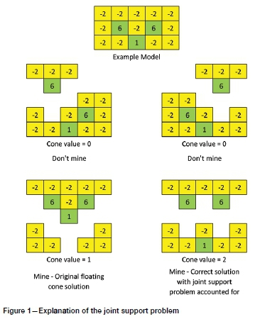
First described by Carlson et al. (1966), the heuristic floating cone algorithm has been widely used in industry due to its simplistic nature, fast running time, and ease of comprehension. As suggested by the name, the algorithm is based on the combined value of all blocks within each cone that is systematically imposed above each block from the top to the bottom of the block model. If the value of a cone is positive, all blocks within the cone are added to the optimal solution, and the algorithm advances to the next block in the model.

As this method looks at each cone in isolation, it is not able to factor in the joint support problem of UPL determination. The joint support problem describes the situation when in isolation, an ore block does not have a high enough value to carry the required waste removal by itself, but the waste may be common to more than one ore block, potentially making it worth mining both, as shown in Figure 1. Due to this, there is no guarantee of an optimal solution. Several methods of modifying this algorithm have been developed in order to counter this limitation, as summarized by Elahi Zenyi, Kakaie, and Yousefi (2011). While these modifications have improved the accuracy of the algorithm, they still do not guarantee the optimal solution as calculated using a rigorous method.

 

 

Dynamic programming

The original dynamic programming algorithm published for solving the UPL problem was by Lerchs and Grossmann (1965). It is designed to work on two-dimensional economic block models, in conjunction with a known set of pit wall angles that provide the dependency relationships between blocks. This algorithm always provides the optimal solution when operating on a two-dimensional block model; however, open pits are three-dimensional. The solution originally presented to extend this method to three dimensions is to complete the algorithm for all vertical cross-sections of the block model, and then reassemble to a complete model. Due to each cross-section being analysed in isolation, they will inevitably not fit together in such a way that maintains all required safe pit wall angles. This results in a need to smooth out the walls in order to meet the pit wall requirements. This smoothing is both time-intensive and subject to error, with the resulting pit contour being far from optimum.

Several algorithms have been developed that have aimed to implement pit optimization using dynamic programming in three dimensions. Due to the complexity of the problem, they often become impractical. Johnson and Mickle (1970) and Johnson and Sharp (1971) conducted some of the earlier work in the area, and maintained a similar algorithm to the two-dimensional approach. However, when evaluating a block, the block value information from the current cross-section and the perpendicular cross-section were taken into account, leading to more accurate results.

Koenigsberg (1982) presented the first example of a truly three-dimensional dynamic programming algorithm to solve the UPL problem. This algorithm considers the relationship between levels within a column, and columns within a cross-section, in addition to the block values from the current section of interest. Though this now gives the ability to work effectively in three dimensions, the algorithm is limited to having generalized wall angle constraints. This means that the pit wall angles must be the same in all directions.

Though there have been various advances in the dynamic programming approach to solving for UPL, it evidently remains impractical to use it accurately in three dimensions, for two reasons; pit wall smoothing from the two-dimensional method, and generalized pit wall angle constraints. Although these algorithms are classified as rigorous, the proof of this shows that they always achieve the optimum for the task assigned. This task does not yet factor in all variables, and as such, the optimum achieved is very rarely the true optimum for the block model.

Lerchs-Grossmann

Lerchs and Grossmann (1965) also proposed an algorithm to solve the UPL problem in three dimensions. The algorithm is based on graph theory, where each node in the graph is representative of a block in the economic block model. This gives each node a weight equal to the economic value of a specific block that it represents. Directed arcs within the graph represent pit wall constraints and dependencies between blocks. Once the graph is set up, solving for the ultimate pit is analogous to solving for the maximum closure. In order to do this, Lerchs and Grossmann developed an algorithm that uses a series of naming conventions that dictate graph tree transformations that in turn solve for the maximum closure, i.e. the UPL.

Due to its ability to use generalized pit slope rules, to work truly in three dimensions, and always return the mathematically provable optimal solution, the graph theory algorithm has become the most commonly used algorithm in UPL optimization, with commercial implementation in several mine planning software packages, including Whittle4X, Datamine Studio 3, and DeswikCAD.

Network flow

In addition to presenting their graph theory algorithm, Lerchs and Grossmann (1965) noted that the UPL problem can be transformed into a network flow situation. In order to do this, the graph theoretic tree is transformed into a bipartite network, with each block in the model represented by a node in the network. Nodes that represent positive value blocks are linked to the source by arcs with capacities equal to the blocks' economic value, while nodes that represent negative value material are linked to the sink by arcs with capacities equal to the absolute value of the blocks' economic value. Dependencies between blocks are represented by joining the positive value blocks to their respective overlying blocks by arcs with infinite capacity. Once this is complete, the UPL is found by solving for the maximum flow/minimum cut of the network.

Like the graph theory algorithm, this method is also able to work with generalized pit slope rules, to work truly in three dimensions, and always return the mathematically provable optimal solution. Two aspects separate this method from the graph theory algorithm, the first being that it is relatively easy to understand in comparison to the graph theory approach. The second is that due to the importance of the solution of general network flow problems in operations research, a great deal of resources has been devoted to the development of efficient computer code to solve for maximum flows (Fox, 1978). The most recent development in solving for maximum flows is the pseudoflow algorithm (Hochbaum, 2008), which is implemented in DeswikCAD for the determination of UPLs.

 

Major differences in pit design

Due to the different operational nature of FMIPCC haulage systems compared with truck haulage systems, there are fundamental differences in the requirements of pit design (Dean et al., 2015). For a truck haulage system, the only requirements for pit design are haul roads providing access to the pit, and that the minimum mining width for the proposed equipment is met. These two requirements do not have any impact on the UPL; therefore, UPL determination can be completed as normal, with pit design to follow.

For FMIPCC systems, there are other requirements for pit design in addition to pit access and the mining width, due to the use of conveyors. For conveyors to work efficiently, they must be used in linear set-ups, similar to a strip-mining operation. This requires mining benches to be mostly regular and horizontally extensive (Atchinson and Morrison, 2011). Due to the nature of conveyor operations, having large horizontal traverses, it is also a requirement to have regularly flat pit floors to facilitate bench conveyor shifts.

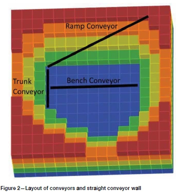
The third requirement is the inclusion of a straight wall for the conveyor to exit the pit. Ideally, this straight wall should be long enough for the conveyor to reach to the top of the pit from the bottom without switching back. If the conveyor is required to switch back on itself, it is recommended that the number of transfer points be minimized due to the inefficiencies that stem from material hangups and spillage (Spilker, Albers, and Lordi, 1980), which lead to an overall reduction in reliability of the series connected system (Frankel, 1984). Figure 2 shows an example pit with the various conveyors indicated. The ramp conveyor is located on the straight conveyor wall which is calculated within presented solutions.

 

 

Partial solutions to FMIPCC UPL determination

Floating trench

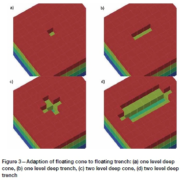
The most basic algorithm to adapt for use with FMIPCC systems is the floating cone algorithm. Its natural extension into working with a straight fixed wall is to lengthen the virtual cone that sequentially floats over a block model to collectively find positive value blocks and thus form a trench (Figure 3). The length of the trench could be modified depending on how many switchbacks of the ramp conveyor on the straight wall are appropriate for the study. This trench would be floated until a positive-value fixed wall location is found, and the traditional cones could be floated to solve for the best pit from this wall location. Following this, the algorithm could be reset, and the trench could find the next positive fixed wall location.

 

 

This floating trench algorithm, though simple, would inherit the generic floating cones' weaknesses, as well as introduce additional problems of its own. As the floating cone algorithm does not require a fixed wall, there is no need to run the algorithm more than once, since if a block is worth taking, it is added to the ultimate pit and the algorithm continues. However, with the introduction of a fixed wall in the form of a trench, the algorithm would have to be run for each potential wall location and orientation. Relocation of the trench and subsequent solving of the problem for each fixed wall location would add considerably to the solution time. This solution time would further increase given that the model would have to be solved for each of the four principal orientations of the block model. A further disadvantage of this potential solution is that taking a step back to an entirely heuristic solution is not justified given that rigorous solutions to the foundation problem exist.

Adaptation and extension of network flow

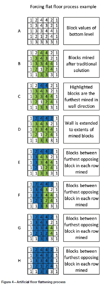
Another proposed solution is to extend the use of a rigorous method with a brute force approach to achieve the additional requirements of FMIPCC systems. This is done by taking the traditional UPL solution and including additional blocks on the lowest level, as described in Figure 4. While the initial solution is a rigorous one (Lerchs-Grossmann or network flow), this method then adds additional blocks to the ultimate pit with no regard for optimality. Due to the process of this algorithm, it is limited to using only the four principal directions of the model.

 

 

Critical analysis of current developments

While both of these proposed developments in FMIPCC UPL determination make some progress towards developing linearly extensive, flat pit floors and a straight fixed footwall, they are both subject to the same two limitations: the inability to calculate an UPL in any orientation for the straight footwall; and the use of non-rigorous methods, reducing the optimality of the results.

With regard to orientation, each of the existing developments can only use the four principal directions of the block model to locate a fixed footwall. As metalliferous deposits exist in any orientation, it is necessary to calculate an orientation that maximizes the potential value, working in the full 360° range.

 

Proposed orientation determination and implementation method

The first item to note when discussing an orientation determination method for FMIPCC UPL calculation is that reverting to a fully heuristic solution is not ideal. For this reason, the proposed solution runs as an extension to the rigorous network flow solution.

Secondly, due to the similarities between strip mining and FMIPCC systems, it is important to highlight that the schedule will closely resemble a stripping operation, radiating from the surface at the location of the straight conveyor wall and progressing across and deeper into the deposit. This in turn means that due to the time value of money, material closest to the surface, and closest to the straight wall where the conveyor is housed, retains more of its value than material further away.

Thirdly, as the size of the UPL increases with depth due to additional waste being removed to access lower ore blocks, the optimal orientation for the UPL may change, depending on how deep the flat pit floor is. As a result, the orientation of the UPL must be calculated for each level of the block model acting as the floor (i.e. limiting the levels which are available for optimization).

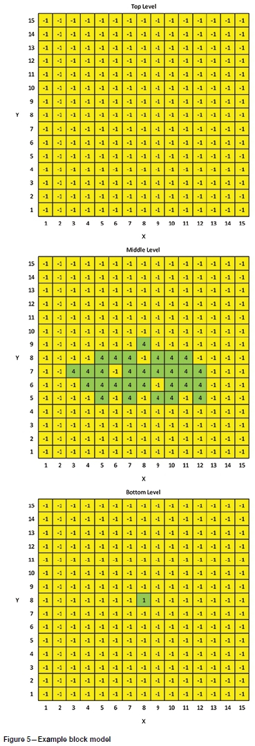
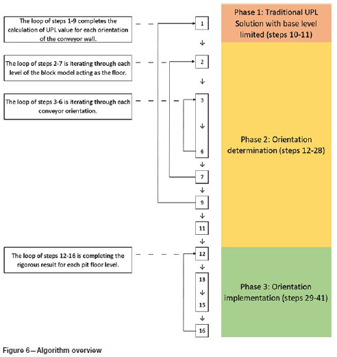
A simple block model is used to highlight processes throughout the algorithm (Figure 5). Although this block model is a simple, small example, the algorithm will operate on larger block models. Waste blocks (yellow) have a cost of -1, while ore blocks (green) have positive values of 1 or 4. The algorithms for orientation determination and implementation are detailed in the following sections, with an overview of the process provided in Figure 6. Note that the bottom level of the example model is omitted from Figures 7 and 8 as it does not form part of the UPLs of any solutions.

 

 

 

 

 

 

 

 

Orientation determination

In order to determine appropriate orientations for FMIPCC UPLs that maximize potential value in the creation of a straight fixed footwall, the user must provide an orientation step size and a discounting rate. The steps used to determine the orientation for any level of the block model are as follows.

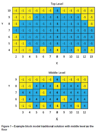
1. Run a standard network flow solution with the level to be used as the flat floor set as the minimum level of the model. This will provide the blocks that are part of the traditional UPL from the surface down to the limiting level. This solution for the middle level being the floor is shown in Figure 7, with blocks that are part of the UPL shown in blue.

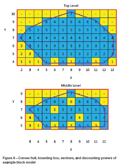
2. Starting with the deepest of the investigated levels, the centroids of the blocks that are part of the UPL are identified and their convex hull is determined. A convex hull is the smallest polygon drawn that contains all points of a set, in which a line drawn between any two points in the set does not protrude outside the convex hull (de Berg et al., 2008). The convex hulls of the top two levels of the example block model's traditional solution are shown in Figure 8 in purple.

3. Rotation (c, current rotation) is set to 0°, the convex hull is rotated anticlockwise by c°.

4. A bounding box is formed around the convex hull, with an additional 0.5 block width distance added to each side/end. This bounding box is rotated c° clockwise to form the bounding box at orientation c° around the original convex hull for the level. Note that the side of the bounding box that is considered the conveyor wall is the side opposite when the current rotation angle is on a compass. The 0° bounding boxes of the top two levels of the example block model are shown in Figure 8 in red.

5. The bounding box is split into sections based on how long its sides are. The number of sections is the next integer below the length, e.g. if the bounding box is 5.4 block widths long and 3.2 block widths wide, it will be split into five sections in the corresponding direction, and three sections in the other. Note that at 0°, the section lines are equal to the block edges.

6. All blocks (ore and waste) within each small section formed by the divisions made in step 5 are attributed a discounting power based on their location with respect to the conveyor wall, and their depth in the model. Blocks that are between the conveyor wall of the bounding box and the convex hull, as well as blocks inside the convex hull, are included in the process. Blocks outside of the convex hull towards other sides of the bounding box are not given a discounting rate, as they are not required to be mined. The value of each block is discounted using the attributed discounting power and user-provided discounting rate to a present value. The sum of blocks on the level is taken and added to the cumulative total for the current orientation. It is important to note that the discounting powers attributed are not derived from an actual schedule, but used to mirror the concept of the time value of money. Figure 8 shows how these discounting powers are attributed for the top two levels of the example block model.

7. Steps 3-6 are repeated for each orientation between 0° and 360° at intervals determined by the user. The step size provided is essentially a control over the resolution at which the user wishes to investigate the model.

8. Once all orientation values are calculated for the current level, steps 2-7 are repeated for each level in the current limited traditional UPL, progressing upwards towards the surface.

9. Steps 1-9 are completed again with each level of the block model being set as the limiting flat floor level.

10. At this stage, the algorithm has a total value for the UPL for each orientation of the straight conveyor wall (including the additional waste requiring extraction to make a straight wall, and flat floor) and for each potential flat floor level. It should be noted that although these values are discounted in the same fashion as present values are for scheduling purposes, it does not reflect a scheduled pit. The discounting is only to mirror the effects of the material being closest to the conveyor wall being worth more than material further away.

11. These total values are scanned, with the maximum value orientation for each flat floor level being highlighted to the user in a list of options to be chosen to run. Multiple orientations on the same level that have the same value will each appear in the list of options as one may be more favourable for geotechnical reasons. Each option is stored with its discounted value, its maximum value orientation, and the level at which the flat floor is located.

Orientation Implementation

Once the orientation determination has been completed, and the user has selected which options to run, each option is implemented and solved using the following steps.

12. Run the standard network flow solution with the minimum level to be used set as the flat floor level of the current option. This will provide the blocks that are part of the traditional UPL from the surface down to the option's flat floor level.

13. The centroids of the blocks which are on the flat floor level of the UPL are used to create a convex hull, bounding box, and sections at the option's orientation, in the same way as was carried out during orientation determination.

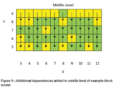
14. Once the sections have been created on the flat floor level, additional dependencies are added to the model from the far side of the model, towards the straight conveyor wall. This provides the model with the additional information required in order to create a flat pit floor and straight conveyor wall. Note that this process is only required to be completed on the lowest level of the option. Figure 9 shows the additional dependencies added to the middle level of the example block model.

 

 

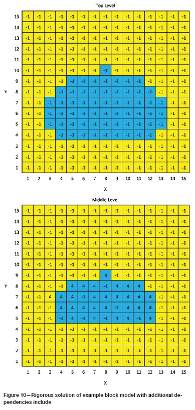
15. This updated model is fed into the network flow solver again, where it is rigorously solved for the FMIPCC UPL, which includes a flat pit floor and a straight conveyor wall. Figure 10 shows the rigorous solution of the example model with the additional dependencies on the middle level included.

 

 

16. Steps 12-15 are completed for each option, with all results being returned to the user in the form of an undiscounted pit value, as expected for an UPL.

 

Discussion

Figure 10 shows the FMIPCC UPL of the example block model. It can be seen that the solution has the required regular flat pit floor and the straight conveyor wall on the bottom edge of the pit. This shows that the proposed algorithm for FMIPCC UPL orientation determination and implementation is successful in achieving the two additional requirements for this small block model.

Figure 10 also shows that block (3,7) on the middle level of the model is not mined as part of the FMIPCC UPL, whereas it is included in the traditional solution. This is due to the two additional blocks of waste that must be mined towards the straight wall in order to include it in the solution. These two blocks, and the three waste blocks above it that would require mining, have a net value of -1. This shows that the flat floor towards the conveyor wall is not being forced to be mined based on the bounding box, but that the final solution remains a rigorous process, resulting in the true optimum for that orientation and depth.

 

Conclusion

Due to the additional requirements of FMIPCC systems that affect the shape of the mine, the mine must be designed around the use of the system. As pit design is based on the input from UPL determination, the additional requirements of FMIPCC systems should be included in the UPL determination stage. In order to do this, a new method of UPL determination must be developed.

The presented method for FMIPCC UPL orientation determination and implementation operates as an extension to a traditional rigorous solution. The first phase uses the results of a rigorous traditional solution as the input, and returns maximum value options with differing depths and orientations. This process is completed by using heuristic methods built around the mathematical concepts of convex hulls and bounding boxes. This is used to implement discounted block values that mirror the time value of money with respect to their location in relation to the conveyor wall, in order to enhance the potential value of the mine. The second phase uses the various maximum value options from the first phase to add additional dependencies to the traditional solution, which are then solved rigorously for each case. This method leads to UPLs that have both regular flat pit floors and a straight conveyor wall. Although the example model used to explain the algorithm is small, the algorithm will operate on larger models. It should be noted that as the block model size increases, the time taken to reach a solution will increase, but as computing power is significantly more advanced now this does not pose a significant problem.

The inclusion of the additional requirements of FMIPCC systems in a UPL determination algorithm advances the ability to optimize and design the mine around the mining system. This work leads directly into testing and verification of the method, with potential avenues in the development of software.

 

Acknowledgments

This work is supported by an Australian Government Research Training Program Scholarship.

 

References

Atchinson, T. and Morrison, D. 2011. In-pit crushing and conveying bench operations. Proceedings of Iron Ore 2011, Perth, 11-13 July. Australasian Institute of Mining and Metallurgy, Melbourne        [ Links ]

Carlson, T.R., Erickson, J.D., O'Brian, D.T., and Pana, M.T. 1966. Computer techniques in mine planning. Mining Engineering, vol. 18, no. 5. pp. 53-56.         [ Links ]

De Berg, Μ., Cheong, o., van Kreveld, Μ., and Overmars, M. 2008. Computational Geometry: Algorithms and Applications. Springer-Verlag, Berlin/Heidelberg. pp. 2-3        [ Links ]

Dean, Μ., Knights, p., Kizil, M.S., and Nehring, Μ. 2015. Selection and planning of fully mobile in-pit crusher and conveyor systems for deep open pit metalliferous applications. Proceedings of the Third International Future Mining Conference, Sydney, Australia, 4-6 November 2015. Australasian Institute of Mining and Metallurgy, Melbourne. pp. 219-225.         [ Links ]

Elahi Zenyi, Ε., Kakaie, R., and Yousefi, A. 2011. A new algorithm for optimum pit design: Floating cone method III. Journal of Mining & Environment, vol. 2, no. 2. pp. 118-125.         [ Links ]

Fox, B.L. 1978. Data structures and computer science techniques in operations research. Operations Research, vol. 26, no. 5. pp. 686-717.         [ Links ]

Frankel, E.G. 1984. Systems Reliability and Risk Analysis. Springer, Dordrecht. The Netherlands. pp. 73-106.         [ Links ]

Hochbaum, D.S. 2008. The Pseudoflow algorithm: a new algorithm for the maximum flow problem. Operations Research, vol. 56, no. 4. pp. 992-1009.         [ Links ]

Johnson, T.B. and Mickle, D.G. 1970. Optimum design of an open pit, an application in uranium. Proceedings of the 9th International Symposium on Techniques for Decision-Making in the Mineral Industry, Montreal, 14-19 June 1970. Canadian Institute of Mining, Metallurgy and Petroleum, Montreal. pp. 331-338.         [ Links ]

Johnson, T.B. and Sharp, W.R. 1971. A three dimensional dynamic programming method for optimal ultimate open pit design. Report of Investigations 7553. US Department of the Interior, Bureau of Mines, Washington.         [ Links ]

Kim, Y.C. 1978. Ultimate pit limit design methodologies using computer models - The state of the art. Mining Engineering, vol. 30, no. 10. pp. 1454-1459.         [ Links ]

Koenigsberg, Ε. 1982. The optimum contours of an open pit mine: an application of dynamic programming. Proceedings of the 17th International Symposium on Application of Computers and Operation Research in the Mineral Industry. Society for Mining, Metallurgy and Exploration, Littleton, CO. pp. 274-287.         [ Links ]

Lerchs, H. and Grossmann, I.F. 1965. Optimum design of open-pit mines, CIM Bulletin, vol. 58. pp. 47-54.         [ Links ]

Nehring, Μ., Knights, p., Kizil, Μ., and Hay, Ε. 2018. A comparison of strategic mine planning approaches for in-pit crushing and conveying, and truck/shovel systems. International Journal of Mining Science and Technology, vol. 28, no. 2. pp. 205-214.         [ Links ]

Spilker, E.C., Albers, T.J., and Lordi, A.c. 1980. Technical aspects of overland belt conveyors. Preprint no. 80-54. Society of Mining Engineers of AIME, Las Vegas, Nevada.         [ Links ]

 

 

Correspondence:
E. Hay
Email: edward.hay@uqconnect.edu.au

Received: 29 Apr. 2018
Revised: 27 Aug. 2019
Accepted: 10 Oct. 2019
Published: November 2019