GENERAL PAPERS

 

A comparative study of lignite resource estimation based on 1D drill-hole mineable lignite compositing of uncorrelated seams and 3D mineable lignite aggregation of correlated seams

 

 

I. Kapageridis; A. Iordanidis

Department of Mineral Resources Engineering, University of Western Macedonia, Koila, Greece

Correspondence

 

 

---

SYNOPSIS

The majority of lignite deposits in Greece consist of multiple thin lignite layers and are traditionally estimated using a one-dimensional compositing approach that can potentially lead to large errors, particularly in the presence of medium to severe tectonic disturbance and uneven vertical distribution of the seams. Drill-holes are evaluated using mining and processing criteria leading to a number of mineable lignite 'packages' along each hole, the sum of which is reported as the total mineable lignite at each drillhole horizontal location. The total mineable lignite thickness values from the various drill-holes and associated weighted average qualities are interpolated horizontally, leading to a two-dimensional model of mineable lignite. A more advanced version of this one-dimensional approach has been applied in the past, with improved results. In this version, the one-dimensional approach was limited to a single mine bench and repeated separately for each bench, thus reducing the scale of potential errors and better approaching the vertical distribution of mineable lignite. Lignite deposits, such as the one examined in this paper, require the development of a thorough stratigraphic model to allow the reporting of accurate lignite resources and to form a solid basis for mine planning and the calculation of lignite reserves. The evaluation of mineable lignite using mining and processing criteria can then be applied to correlated and modelled lignite seams, leading to an overall three-dimensional model of the deposit that allows accurate calculation of lignite resources even in the presence of deformation. This paper presents all three modelling approaches through a case study based on part of a real lignite deposit. The effects of using each of the approaches are analysed and the benefits of the three-dimensional approach are clearly demonstrated.

Keywords: resource estimation, drill-hole data, compositing, aggregation, correlation.

---

 

 

Introduction

The modelling problem

Coal and other stratiform deposits consisting of multiple layers require a lot of time and effort to produce a representative geological model that will allow accurate estimation of resources and provide a solid basis for effective mine planning. The transition from such a 3D geological model of stratigraphy to an effective run-of-mine model that can be used to calculate reserves is a critical part of this process. Approaches to achieve this transition range from one-dimensional mineable coal compositing of drill-hole data to more effective three-dimensional aggregation of mineable coal seams based on an appropriate stratigraphic model. Coal and lignite resource modelling has been covered in a number of studies (Tercan and Karayigit, 2001; Heriawan and Koike, 2008a, 2008b; Kapageridis and Kolovos, 2009; Olea et at., 2011 ; Hatton and Fardell, 2012; Roumpos, Liakoura, and Barmpas, 2011, 2014; Tercan, Ünver, and Hindistan, 2011; Deutsch and Wilde, 2013; Tercan et al., 2013)

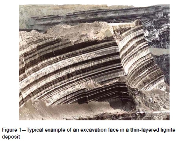
Thin-layered lignite deposits (known as Zebra deposits) are the main source of fuel for the production of electrical power in Greece (Figure 1). Mainly located in the northwest region of the country, in the Amyntaio-Ptolemais basin, Greek lignite deposits belong to the upper Pliocene. Overburden material belongs to the Pleistocene and Holocene (Anastasopoulos and Koykoyzas, 1972). Over the lignite-bearing strata lies a series of green-gray clay and marl layers - an alternation of mainly sandy clays, calcareous marls, and silty clayish marls. A series of yellow-brown sandy layers follows, consisting of mainly calcareous sands with clay intercalations and occasionally sandy marls. In this formation, numerous lenticular intercalations of sandstones and consolidated conglomerates exist. Over the yellow-brown layers lies a series of red-brown clays and conglomerates - an alternation of reddish sandy clays and poorly consolidated conglomerates with clay-silica matrix.

 

 

The large number of lignite layers combined with the complexity of their spatial distribution, and the large number of drill-holes from different campaigns analysed by different people and using different methodologies, has led to the adoption of an over-simplistic approach for the estimation of resources and reserves of these deposits. Locally developed software used for this purpose since the early 1990s (and still in use today) is based on a one-dimensional compositing approach (referred to as 1D mineable intervals). Each drill-hole is composited using mining and quality criteria forming mineable lignite sections, the sum of which is reported as the total mineable lignite at the drill-hole horizontal location. The total mineable lignite values from the various drill-holes are interpolated horizontally, leading to a two-dimensional grid model of the mineable lignite parameter. This approach is capable of calculating global lignite resources with acceptable accuracy provided the sample density is sufficiently high. However, it is particularly prone to errors in calculating local lignite resources, which are necessary for effectively planning and scheduling a continuous mining process. Another issue with this approach is the sensitivity of the results to potentially incomplete or incorrectly interpreted drill-holes which, due to the one-dimensional nature of the modelling process, can lead to significant errors in local resource estimates.

A further development of the 1D mineable intervals method was introduced and adopted in 2012, partially solving the problem of over-generalizing the vertical distribution of mineable lignite by splitting its thickness per bench. In other words, the mineable lignite intervals produced by the previous method are split and coded by bench - each bench is considered as a separate 'deposit' with its own mineable lignite, overburden, midburden, and underburden thicknesses and lignite qualities. This approach (referred to as 1D bench mineable intervals) is a significant improvement over the previous method, but close examination of the produced models revealed similar issues as before, although on a smaller scale. The aim of this paper is to clearly present these issues, relate them to the lack of a complete stratigraphic model of seam correlation, and demonstrate how such a model would resolve them and form the basis for accurate and more detailed lignite reserve estimation and mine planning. In summary, three methods of lignite resource estimation are discussed and compared:

1. One-dimensional compositing of total drill-hole mineable lignite intervals-ID mineable intervals method

2. One-dimensional compositing of drill-hole mineable lignite intervals per bench-1D bench mineable intervals method

3. Three-dimensional mineable lignite aggregation of correlated lignite seams.

Example data-set

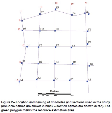
Data used to compare the lignite resource modelling approaches in this paper comes from an exhausted lignite mine in NW Greece. A small area of the mine was selected containing a total of 24 drill-holes on a random grid of 5 χ 5 m (Figure 2). The model limits cover an area of 1.32 km². The names and coordinates of the drill-holes have been changed for confidentiality purposes. The area topography was not used in the study for the same reason - the drill-hole collar was taken as the top of overburden (excluding drill-hole C5). Reported resources were limited only by the study area polygon - no pit surface was used in the study. Figure 2 shows the drill-hole collar locations in plan view. Drill-holes were named according to their row and column number, which correspond to the section names. For example, drill-hole A1 is located in section A and section 1. The 24 drill-holes comprised a total of 2950 original (raw) intervals. The data-set was imported to a database and validated.

 

 

One-dimensional compositing of total drill-hole mineable lignite intervals - 1D mineable intervals method

Method

The method for compositing drill-hole mineable intervals described in this section is very similar to the one applied to Greek lignite deposits (Karamalikis, 1992). The method used in this paper employs the integrated Mineable Intervals option in Maptek Vulcan software plus some extra steps before and after applying this option to make it more suitable for lignite seams. A comparative study has been performed in the past to prove the similarity of the results produced by this approach and by the software traditionally used for compositing of Greek lignite deposits (Kapageridis, 2006). The method is applied using the following steps.

> Pass 1: The program looks at samples down the hole and classifies each sample as lignite or waste based on the ash cut-off value specified.

> Pass 2: The program combines adjacent samples of lignite and waste to produce runs of pure lignite and pure waste.

> Pass 3: Working from the top of the hole down, the program checks if the waste interval between the first lignite run and the subsequent lignite run is shorter than the waste absorption maximum length. If the waste length is longer than this limit, then the lignite runs are left as separate composites and the waste length from the second lignite run to the third is checked. If the waste length is shorter than the limit, then the first lignite run, the waste run, and the second lignite run are added together, and the resulting ash value is computed. If the ash value

is higher than the lignite/waste cut-off value, then the lignite and waste runs are left as individual composites and the process moves on to the second and third lignite runs. If the resulting ash value is lower that lignite/waste cut-off value, then the interval is accepted as a single lignite composite. The waste length between this new lignite composite and the subsequent lignite run is then checked, and the process described above is repeated.

> Pass 4: At this stage there are lignite runs that incorporate internal waste where possible and whose ash value is below the lignite/waste cut-off value. The procedure then continues to add upper and lower waste dilution to these lignite runs. It will add adjacent waste samples up to a specified dilution length. It should be noted that this step will not disqualify any lignite runs. Roof and floor losses are applied to lignite intervals and respective gains to waste intervals.

> Pass 5: The final pass checks all resulting lignite runs to see if they are longer than the minimum lignite run length. Lignite runs that are shorter than this limit are reclassified as waste and absorbed into the surrounding waste runs. All quality calculations are length-weighted.

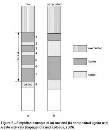
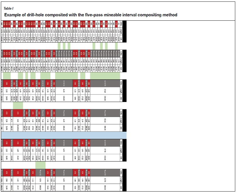
Figure 3 shows a simplified example of the input (raw) and output (composited) version of a drill-hole using the mineable intervals compositing method (Kapageridis and Kolovos, 2009). Lignite and waste raw intervals are combined to form mineable lignite or waste composited intervals based on criteria such as minimum lignite thickness, maximum waste absorption thickness, mineable lignite ash upper limit (cut-off), and mineable lignite roof and floor losses and dilution.

 

 

Compositing

Applying this method to the 24 drill-holes of the example data-set led to the generation of 1016 composited mineable intervals of lignite and waste from the 2950 raw intervals. The generated composites table was added to the original drill-hole database. Table I presents the output of each of the five passes of the mineable intervals compositing method on part of a drill-hole from the data-set. Lignite intervals at each pass are coded as CO. Waste horizons are coded as WASTE after the first pass. Only part of the drill-hole is shown in the table. The total length (thickness) of mineable lignite per drill-hole was calculated next. This was stored together with other information such as the top and bottom depth of mineable lignite in a formatted text file. The file contained information on the thickness and depths of overburden and midburden. These files were used to calculate and locate lignite resources within the study area limits. A 0.5 m minimum mineable lignite thickness and 0.3 m waste thickness were applied. The maximum ash content for lignite was set to 36% and the roof and floor losses for lignite were 0.1 m.

Resource modelling

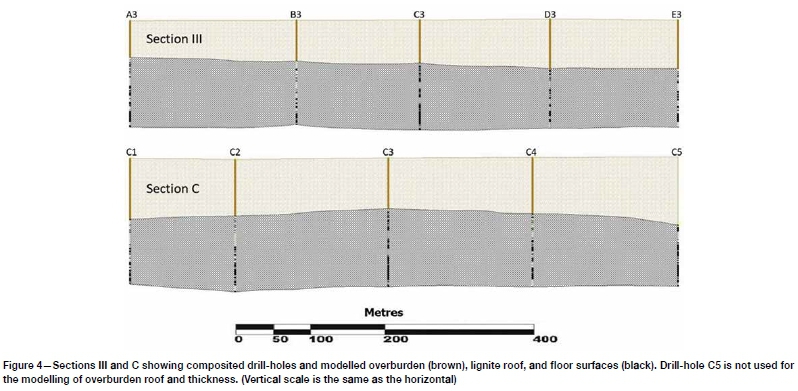
Using the information contained in the formatted text files for the thickness, roof, and floor of the mineable lignite and the corresponding values for overburden and midburden, grid models were generated using the inverse distance weighting method. The power of 1 for inverse distance was used for the roof and floor models, while the power of 2 was used to model thicknesses. Figure 4 shows sections III and C, which cross through the middle of the study area - the overburden is clearly displayed as a single layer, while lignite and midburden are shown together. The lack of seam correlation means that it is not possible to display (and model) lignite seams as separate layers in section.

As the lignite seams are not correlated, we rely on the total mineable lignite thickness model for resource estimation. The stripping ratio is also calculated using the total overburden and midburden thickness models. Calculating lignite resources per bench are based on the total mineable midburden/lignite ratio and the thickness of their sum (lignite plus midburden) within each bench. The same midburden/lignite ratio is effectively applied to all benches, with the only possible varying parameter being the thickness of the mineable lignite plus midburden. For benches totally enclosed in the area between the roof and floor of mineable lignite, this parameter is constant, leading to equal resources being reported in these benches.

 

One-dimensional compositing of drill-hole mineable lignite intervals per bench - 1D bench mineable intervals method

Method

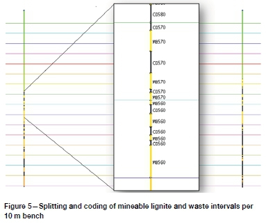
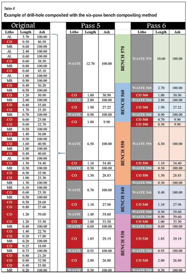
The second approach considered is based on the five-pass compositing method discussed in the previous section, but adds an extra pass where the produced lignite and waste composite intervals are split and coded based on surfaces corresponding to mining benches (Figure 5). The height of the benches can be constant or differ between benches, and essentially controls the vertical resolution of the calculation. As the interval splitting takes place after any quality- and thickness-based classification to lignite or waste, the added sixth pass does not reduce the total mineable lignite of a drill-hole calculated by the previous method. It simply distributes the mineable lignite and waste to separate benches, allowing the more accurate calculation of resources per bench. Mineable lignite or waste composite intervals vertically crossing the floor of a bench are split in two components, each coded according to the bench volume they belong to (e.g. CO560, CO570, etc.). This approach was used in the lignite resources estimation and mine planning study of the Mavropigi Field (Public Power Corporation of Greece) in 2012.

 

 

Compositing

The 1016 mineable lignite and waste composite intervals from the previous method were intersected with bench surfaces every 10 m vertically (pass 6). This led to the generation of 1404 new composites that were stored in a separate table of the database. Table II shows how this was done on the same part of the drillhole presented in Table I.

The total length (thickness) of mineable lignite per drillhole and bench was calculated next. This information was stored, together with other information such as the top and bottom depths of mineable lignite within each bench, in separate formatted text files - one per bench. The files contained information on the thickness and depths of overburden and midburden in each bench. These files were used to calculate and locate lignite resources within the study area limits for each bench.

Resource modelling

The same process followed in the previous method, was applied in the case of mineable lignite composites per bench. The formatted text files were used to generate grid models of the roof, floor, and thickness of mineable lignite, overburden, and midburden. This time, there were several models corresponding to the different benches, and resources were calculated per bench using the composited mineable thicknesses per bench. There was no need to use the waste to lignite ratio to calculate resources per bench, as the mineable overburden, midburden, and lignite thicknesses were calculated directly for each bench using values related to each bench.

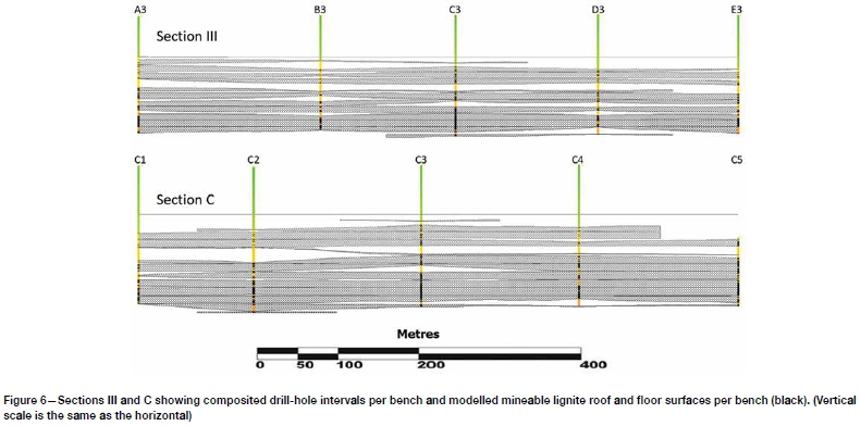
The horizontal extents of mineable lignite in each bench had to be considered during modelling. Vertical variations in lignite density meant that not all drill-holes contained mineable lignite in each bench. This was addressed by applying polygonal masks to the grid models, limiting their horizontal extents as shown in Figure 6. This approach allowed the bench mineable lignite models to maintain their interpolated thickness at their edges, potentially leading to overestimation of mineable lignite resources.

 

Three-dimensional mineable lignite aggregation of correlated lignite seams

Lignite seam correlation

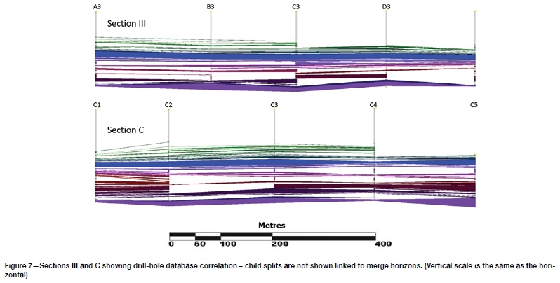
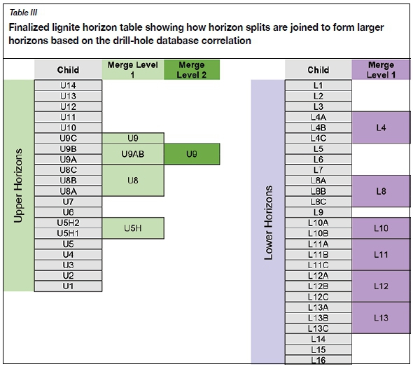
The last method considered in our study was based on the geological analysis, correlation, and modelling of the original (raw) lignite seams. The lignite seams were examined in cross-section and were manually correlated by selecting the drill-hole intervals considered to belong to a particular seam and coding an appropriate seam field in the database. This was a fairly difficult and time-consuming process, the results of which were influenced to some degree by the geologist's interpretation. A number of parameters were used to control correlation of lignite seams, including material colour, location relative to characteristic marl and sand horizons, fossil content, cohesion, friability, and characteristics of surrounding marl horizons. Figure 7 shows drill-hole sections III and C with the seam codes stored in the database after correlation. This type of section helps to visualize the way correlation works before actual modelling of the seams. The software automatically links intervals with the same seam code between successive drill-holes in a linear fashion, aiding the user during correlation. A colour legend helps distinguish between seams as in our case there were so many that the section would become very confusing to the eye. Linking of correlated seams is not allowed through drill-holes that don't contain them. Two characteristic marl horizons were used to group the lignite layers into upper and lower horizons. Upper horizons were numbered upwards (the lowest being U1) and lower horizons were named downwards (the top one being L1). There was no particular reason for this convention other than the need to have a standard convention between drill-holes. Horizon splits were named after the merging horizon, e.g. splits U8A, U8B, and U8C merge to U8 (Table III).

All lignite seam codes and related splits were stored in a special database table and field to be used for structural modelling of the seams. A horizon list (table) was also stored for reference by other functions of the software. The horizon list should only contain stratigraphy that will be modelled. It is important to list the horizons in proper stratigraphic order with the first horizon being the uppermost deposit and the last horizon being the bottom of the modelling area of interest. The smallest split is defined in the 'child split' column. Child splits are merged into larger horizons until the parent horizon is reached on the right-hand side of the table. Horizons with no splitting are also listed in the child split column. Table III shows the horizon list and splits for our case study. The table is presented in two parts -one for the upper horizons and one for the lower.

There were cases of very thin seams that occurred in only one drill-hole, and a drill-hole that was missing most of the upper lignite seams (C5). These and other stratigraphy issues were resolved using a special operation in Maptek Vulcan called FixDHD, which we discuss in the following section. FixDHD is one of the first steps in the modelling procedure called Integrated Stratigraphic Modelling (ISM).

Validating and fixing seam correlation

Data for stratigraphic modelling, as in our case study, is provided from a drill-hole database, with the horizons of interest noted. It is rarely possible to clearly identify all horizons in every hole. This may be due to:

> The geological nature of the deposit being drilled

> Biases introduced when planning the drilling programme

> Poor logging practice

> Lost data.

Our data-set, even though limited to a small area of a much larger deposit and consisting of only 24 drill-holes, presented the following data collection issues that need to be addressed.

> Short holes, which are not deep enough to include all horizons of interest or have a collar lower than the original topography surface

> Difficulty determining the position of missing horizons that have thinned to zero thickness

> Issues determining the position of daughter horizon boundaries within their merged parent horizon.

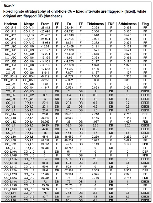
FixDHD was called to check the correlated lignite stratigraphy and fix possible problems. Several problems were initially identified that were preventing the software from resolving the issues. These were problems related to the way correlation was coded (e.g. wrong seam sequence or seams occurring in only one drill-hole). In every trial run, the software produced a detailed log file that explained the issues and suggested ways to resolve them. Once these problems were addressed, a fixed version of the lignite stratigraphy table was produced in the database. Table IV shows how this table looks for drill-hole C5.

The horizons are shown from top to bottom in the fixed table. As drill-hole C5 was missing the top part of stratigraphy, several intervals were interpolated above its collar, shown with a negative From and To relative depth. Intervals interpolated or otherwise fixed are flagged with an 'F' next to the column that was fixed (from, to, or thickness). Intervals unaltered in the fixing process are flagged 'DB'. The final Flag column summarizes the changes associated with an interval. For example, an interval with the original From value (column FF = DB) and a fixed To value (column TF = F) will have a final flag DBF (column Flag). Intervals with no changes are highlighted with light green in the table. The software applies statistical modelling techniques to restore missing or unavailable data from the stored stratigraphy and manipulates the available data to meet required criteria for modelling. If insufficient data is available to apply this technique, less rigorous stacking methods are used. Similar changes to those shown for C5 took place in other drill-holes, leading to a fixed correlation that could be effectively modelled. The fixed version of the database was compared against the original in the database editor (in tabular format) and visually in sections showing database correlation.

Structural modelling

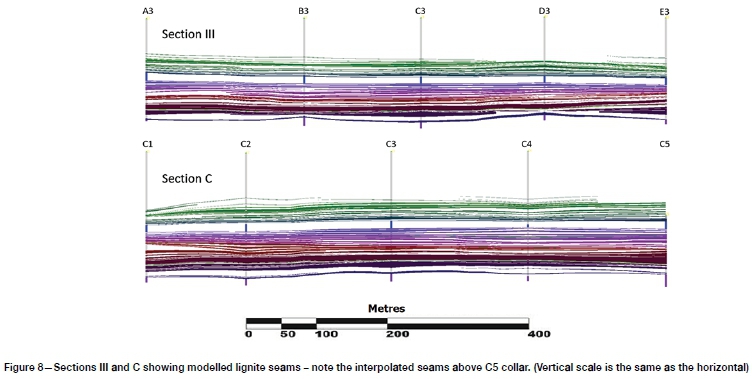
Once the fixed lignite stratigraphic table was produced, structural modelling of the lignite seams could be performed. Seam persistence limits were generated to control the horizontal area of the seams of the fixed lignite intervals. The same interpolation method was used (inverse distance weighting with a power of one) as previously for consistency. Grid models for the roof, floor, and thickness of each seam were generated and masked with the corresponding seam limits. Figure 8 shows sections III and C with the modelled seams. It should be noted that no minimum seam thickness or quality criteria have been applied up to this stage. After roof and floor models for each horizon were created, thickness grids were automatically generated between adjacent pairs of surfaces. Every node in each thickness grid was forced to a value of zero or greater, which ensured that no horizons crossed. Should a horizon cross its neighbour, either the floor was forced to the roof position, or the roof was forced to the floor position.

Compositing and quality modelling

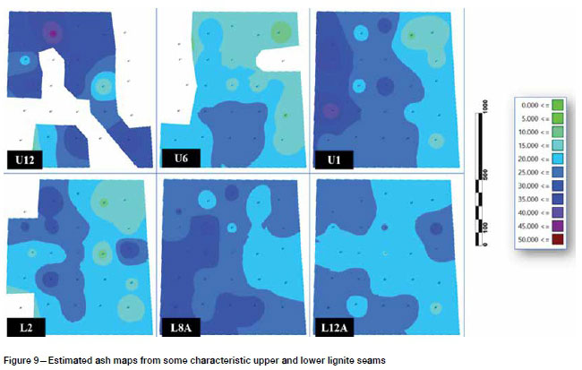
For each of the modelled seams, it was necessary to generate corresponding quality grids, one for each of the quality parameters (ash, moisture, calorific value). Inverse distance weighting to the power of two was used to interpolate composited quality values (single value per seam and drill-hole) to the respective grid models. Figure 9 shows ash contour maps for some lignite seams. Estimating quality parameters separately for each seam leads to a much more detailed quality model than the previous two methods and allows the application of quality mineability criteria in three dimensions instead of one.

Resource model development

The resource model was based on the HARP (horizon adaptive rectangular prism) structure - a type of block model that represents an entire integrated stratigraphic model. The HARP model is created directly from grids or faulted triangulations. All quality grids are automatically incorporated. A HARP model block contains five points in the roof of the block and five points in the block floor (Maptek, 2016). These points allow vertex angles to fluctuate, which allows the block to conform to structure roof and floor grids. HARP models accurately resolve horizons down to a few centimetres of thickness without the need to make huge models with extremely small Z sub-blocking.

All structural and quality grids generated for the modelled lignite seams of our study were used to construct a HARP model using the horizontal extents of the considered area. Each HARP block was initially coded as lignite or waste and allocated a seam code based on the formulated horizon list. Waste block seam codes had a prefix added to distinguish them from lignite (e.g. BD_L7 for burden block above L7). Figure 10 shows two sections through the produced HARP model coloured by ash estimates. It is quite clear that the HARP structure allows the model to follow precisely the modelled stratigraphy.

 

Generation of run-of-mine model

Run-of-mine (ROM) modelling in Maptek Vulcan simulates the way in which material is extracted from a stratiform deposit. Basic parameters are defined for extraction. The ROM HARP model is constructed from the geological HARP model using three rules, applied to the mine modelling process in the following order (Maptek, 2018):

1. Minimum mining thickness: Any horizon less than this thickness is not mined by itself.

2. Minimum parting thickness: Any waste material between seams less than this thickness is mined with the next seam, resulting in composited seams. Waste material becomes a parting in the composited seam. The assumption when using this option is that burden material less than this thickness cannot be separated in the pit, so it is mined with the product. However, compositing only takes place if the minimum product to waste ratio is met.

3. Minimum product to waste ratio: The total product to total waste ratio in a working section must be greater than or equal to this ratio. Total waste is defined as all in-seam partings plus all between-seam parting.

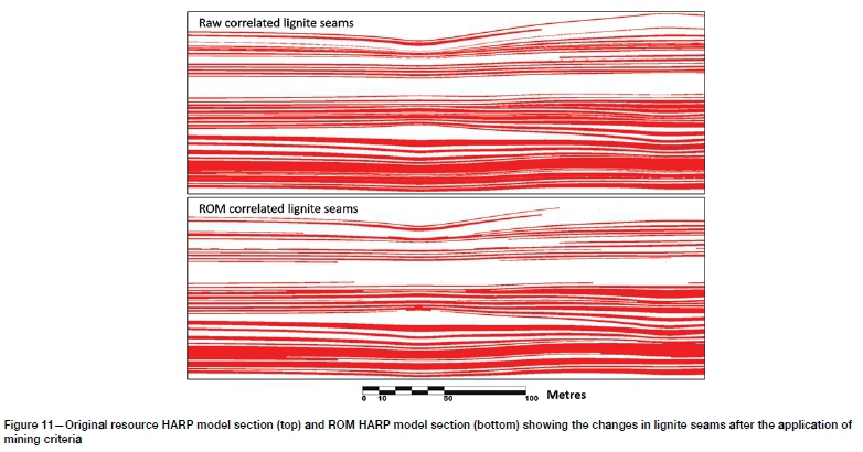
In our study, the minimum mining thickness was set to 0.5 m and the minimum parting thickness to 0.3 m. A 0.1 m roof and floor loss was also applied. Figure 11 compares two sections of the original (resource) and ROM HARP model showing the effect of applying mining criteria to lignite seams in three dimensions. Parts of seams disappear due to thickness criteria and others are combined to form thicker mineable sections.

 

Results and discussion

The three methods compared in this paper were applied to the same data-set, using the same mine planning software package. Timewise, the first and simplest method of the three, the compositing of mineable of total drill-hole mineable lignite intervals, was the fastest to implement (a couple of hours). The number of drill-holes used plays almost no role to the time required by this method. It was also very easy to set up and run. The produced models and information take the smallest amount of hard disk space.

The second method, compositing of drill-hole mineable lignite intervals per bench, required more time than the first method as the process was repeated for each bench considered (4-5 hours altogether). It required an extra compositing step to split the composites of the previous method by bench, and the development of a more complex reserve model based on sets of grids per bench. As all steps are fully automated, this method was still very easy to set up and run.

The third and most complex method, mineable lignite compositing of correlated seams, required correlation of lignite seams between drill-holes - a step that took a couple of days to complete for the 24 drill-holes of our case study data-set. It is quite impossible to estimate how much time it would take to correlate 100 drill-holes or more as it would depend on other factors such as faulting, which did not affect the area considered in this study. Once correlation was complete, the other steps took little time to set up and run - a total of 4 hours to get the final ROM HARP model after correlation.

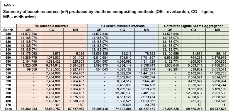
Table V summarizes the resources calculated using each of the three methods. The resources are split by bench, with the waste quantities given in cubic metres while lignite is given in tons assuming a 1.2 t/m³ specific gravity. Looking at the totals, it is clear that the higher the resolution of the calculation (going from method 1 to 3) the lower the reported total lignite. However, looking at the individual benches, the only real comparison can be made between method 2 and 3, as with the first method there is no real control over what is reported as bench quantities. Calculating bench resources using method 1 essentially involves applying the same stripping ratio on a different lignite plus midburden total to derive the individual values. Only overburden can be directly calculated from its modelled floor.

Both methods 2 and 3 report reasonably distributed quantities per bench, but we can still see differences between them. The effect of artificially grouping lignite intervals into bench mineable sections leads to a slight overestimation in the lower benches and some underestimation of the upper ones compared to the numbers reported by method 3. In other words, the more detailed and geology-driven model of the lignite seams that method 3 is based on produces more accurate results than the simplistic mineable lignite model of method 2. These differences could have been much larger if faulting were present. Comparison of quality parameters estimations gave similar differences.

 

Conclusions and future work

Overall, it became quite clear during this exercise that the time taken in building a complete stratigraphic model based on lignite seam correlation is time well spent as it provides all the necessary quantity and quality information in three dimensions and at the highest resolution possible based on the available data. Any efforts to replace seam correlation and compositing with one-dimensional compositing of each drill-hole separately lead to over-simplification of the geology and a significant reduction of the effectiveness of mine planning.

Future work will include the application of all three methods to a mined-out area of the deposit where production figures are well-known and comparison with actual lignite reserves is possible. The implementation of a geostatistical approach to lignite quality parameters interpolation is also one of the improvements planned to the current methodologies.

Finally, the authors recommend that additional drilling could help increase the reliability of resource estimates, regardless of the estimation procedure used, particularly in areas where tectonism and other post-depositional factors have significant effect. Future drilling and drill-hole logging should also be more systematic, with more detailed descriptions and photography of the cores to help in geology correlation modelling and lead to better resource estimates. More systematic logging would also allow the automation of the modelling process.

 

References

ÀNASTAsopouLos, J. and Koykoyzas, C. 1972. Economic geology of the southern part of Ptolemais Lignite Basin (Macedonia - Greece). Institute for Geology and Subsurface Research, Athens.         [ Links ]

Deutsch, C.V. and Wilde, B.J. 2013. Modeling multiple coal seams using signed distance functions and global kriging. International Journal of Coal Geology, vol. 112. pp. 87-93.         [ Links ]

Hatton, W. and Fardell, A. 2012. New discoveries of coal in Mozambique-development of the coal resource estimation methodology for International Resource Reporting Standards. International Journal of Coal Geology, vol. 89, no. 1. pp. 2-12.         [ Links ]

Heriawan, M.N. and Koike, K. 2008a. Identifying spatial heterogenity of coal resource quality in a multilayer coal deposit by multivariate geostatistics. International Journal of Coal Geology, vol. 73, no. 3-4. pp. 307-330.         [ Links ]

Heriawan, M.N. and Koike, K. 2008b. Uncertainty assessment of coal tonnage by spatial modelling of seam distribution and coal quality. International Journal of Coal Geology, vol. 76, no. 3. pp. 217-226.         [ Links ]

Kapageridis, I. 2006. VULCAN 3D software application study on drillhole evaluation. Maptek/KRJA Systems Ltd.         [ Links ]

Kapageridis, I. and Kolovos, C. 2009. Modelling and resource estimation of a thin-layered lignite deposit. Proceedings of the 34th International Symposium on the Application of Computers and Operations Research in the Minerals Industries (APCOM 2009), Vancouver. Curran, Red Hook, NY. https://www.semanticscholar.org/paper/Modelling-and-Resource-Estimation-of-a-Thin-Layered-Kapageridis-Kolovos/c6202d937dda43c3d477ed5fd401c3d7a5b29526        [ Links ]

Karamalikis, N. 1992. Computer software for the evaluation of lignite deposits. OryktosPloutos (Mineral Wealth), vol. 76. pp. 39-50 [in Greek].         [ Links ]

Maptek Pty Ltd. 2016. ISM stratified geologic modelling, Maptek Vulcan training manual. Adelaide, Australia.         [ Links ]

Maptek Pty Ltd. 2018. Integrated Stratigraphic Modelling, Maptek Vulcan 10.1 online help.         [ Links ]

Roumpos, C., Liakoura, K., and Barmpas, T. 2011. Estimation of exploitable reserves in multilayer lignite deposits by applying mining software - The significant impact of geological strata correlation. Proceedings of the 17th Meeting of the Association of European Geological Societies (MAEGS), Belgrade, Serbia, September 14-18. pp. 247-250.         [ Links ]

Roumpos, C., Paraskevis, N., Galetakis, M., and Michalakopoulos, T. 2014. Mineable lignite reserves estimation in continuous surface Mining. Proceedings of the 12th International Symposium Continuous Surface Mining - Aachen 2014. Lecture Notes in Producti_.on Engineering 2015. Springer International.         [ Links ]

Tercan, A.E. and Karayigt, A.I. 2001. Estimation of lignite reserve in the Kalburçaym field, Kangal basin, Sivas, Turkey. International Journal of Coal Geology, vol. 47, no. 2. pp. 91-100.         [ Links ]

Tercan, A.E., Ünver, B., and Hindistan, M.A. 2011. Lignite resource estimation by unwrinkling. Proceedings of the 22nd World Mining Congress and Exhibition., 11-16 September 2011: Proceedings Book, vol. 11. Aydogdu ofset, Ankara-Turkey. pp. 139-142.         [ Links ]

Tercan, A.E., Ünver, B., Hindistan, M.A., Ertunç, G., Atalay, F., Ünal, S., and Killiogu, Y. 2013. Seam modeling and resource estimation in the coalfields of western Anatolia. International Journal of Coal Geology, vol. 112. pp. 94-106.         [ Links ]

 

 

Correspondence:
I. Kapageridis
Email: ioannis.kapageridis@gmail.com

Received: 10 Jan. 2019
Revised: 8 Aug. 2019
Accepted: 10 Oct. 2019
Published: November 2019