GENERAL PAPERS

 

Mineral Resources classification of a nickel laterite deposit: Comparison between conditional simulations and specific areas

 

 

F. Isatelle; J. Rivoirard

MINES ParisTech, PSL University, Centre de Géosciences, France

Correspondence

 

 

---

SYNOPSIS

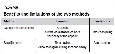
Classification of Mineral Resources as Measured, Indicated, or Inferred depends on the level of confidence the resource geologist has in the estimation of the deposit. This is based on different factors such as the geological or geometrical model, the sampling quality and, from the geostatistical point of view, the distance between drill-holes. However, many methods or criteria used for classification, geometrical ones for instance, are not based on an actual measure of uncertainty. In the present case, which corresponds to a nickel laterite deposit studied in two dimensions, Mineral Resources are classified based on the drilling mesh, and associated probabilities that nominal productions do not deviate from estimations by more than 15%. In this paper we present two methods to assess such probabilities: conditional simulations and the specific areas method. Both methods include the drilling mesh and the spatial variability as principal components for classification and both yield similar results, which allows the validation of one with the other. Benefits and limitations of these two methods are also given. Simulations are time-consuming, but they are the most accurate; specific areas are time-saving and less restrictive for testing several drilling meshes, but the results are more approximate.

Keywords: Mineral Resource classification, conditional simulations, specific areas, nickel accumulation, coefficient of variation.

---

 

 

Introduction

This study deals with classifying Mineral Resources of a nickel laterite deposit in New Caledonia. In mining activities, an area is first classified as Mineral Resources or Reserves, and these are then further classified as Inferred/Indicated/Measured for Resources and Probable/Proven for Reserves. The NI 43-101 (CIM, 2011) states that 'Mineral Resources are sub-divided, in order of increasing geological confidence, into Inferred, Indicated and Measured categories. An Inferred Mineral Resource has a lower level of confidence than that applied to an Indicated Mineral Resource. An Indicated Mineral Resource has a higher level of confidence than an Inferred Mineral Resource but has a lower level of confidence than a Measured Mineral Resource'. While all international reporting codes require a strong Mineral Resources classification, the criteria for defining such classifications are numerous. Besides the geological or geometrical model and the sampling quality, some of the most used criteria are the distance between drill-holes (drilling mesh) and the spatial variability (variogram) of the elements of interest. However, many methods or criteria used for classification, geometrical ones for instance, are not based on an actual measure of uncertainty (Rossi and Deutsch, 2014). Geostatistical methods should then be preferred for classifying Mineral Resources as Measured, Indicated, or Inferred. In the present study, the definition used by the company for Measured Resources is: '90% probability to be within a deviation of ± 15% of a quarter of production', and for Indicated Resources: '90% probability to be within a deviation of ± 15% of a year of production'. To validate the application of this rule to the present case, it is necessary to assess those probabilities objectively with the use of geostatistical methods. The aim of this study is to use and compare two methods for classifying resources from the geostatistical point of view, that is, with respect to the drilling mesh, conditional simulations, advocated by Dohm (2005), and specific areas, presented later in this paper. The remaining sections are devoted to the description of the data-set, the methods, the results, the proposed classification, and a discussion. The study was done in two dimensions and focused on metal accumulations and thickness. The study used Isatis© software (Geovariances, 2017).

 

Data-set and description

The data-set comprises more than 3000 vertical, screened core drill-holes that cover an area of 2.3 km west-east and 1.6 km north-south. Drill-holes are regularly spaced at 25 m; locally drilling has taken place based on meshes of 12.5 m χ 12.5 m and 50 m χ 50 m.

New Caledonia is a large ophiolitic complex formed 35 Ma ago by obduction of the Australian Plate over the Pacific Plate. The deposit is a nickel laterite deposit formed by serpentinization (hydration of the peridotite) and lateritization in a tropical climate (supergene enrichment).

The lateritic profile is divided into six layers that are, from bottom to top:

> Bedrock: peridotite (mainly dunite or harzburgite)

> Rocky saprolite: silicate product of the alteration that is a little weathered

> Earthy saprolite: silicate product of the alteration that is highly weathered

> Transition zone

> Yellow limonite: oxide product of the alteration, enriched in goethite

> Red limonite: oxide product of the alteration, enriched in haematite

> Iron cap and iron shots.

Only the earthy saprolite, the transition zone, and the yellow limonite are mineralized and exploited.

The quarterly production areas for those three layers are given in Table I.

 

 

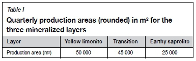
Six variables of interest from a mining and processing perspective were taken into consideration. This paper focuses on nickel (Ni) and manganese oxide (MnO) accumulations. Nickel is extracted by a hydrometallurgical process that requires tight control on the chemistry of the ore fed to the plant. Some auxiliary constituents, like MnO, play a significant role in the recovery of the nickel.

 

Methods

Two methods were used and compared to classify Mineral Resources: conditional simulations (Chiles and Delfiner, 2012) and the specific areas method (Rivoirard and Renard, 2016; Rivoirard et al., 2016).

Conditional simulations coupled with kriging are used to test the ±15% rule. All the variables will be treated conjointly, and cosimulations and cokriging will be run.

The cokriging represents the planned production values while the cosimulations represent the set of the possible real values that will be compared with the cokriging: if 90% of the cosimulations are within ±15% of the cokriging, the Mineral Resources will be classified as Measured or Indicated. If the comparison is done on areas representing a quarter of a year's production, this will satisfy Measured Resources, while a comparison done on areas equivalent to a year of production satisfies Indicated Resources. Production areas are represented arbitrarily but conveniently as squares with the areas given above.

To test the category of Mineral Resource according to the drilling mesh, five drilling meshes were used as inputs: 25 m χ 25 m, 50 m χ 50 m, 75 m χ 75 m, 100 m χ 100 m, and 125 m χ 125 m. Drilling meshes greater than 25 m χ 25 m were created artificially by migrating the drill-holes over grids with size equal to the desired mesh. As the original grid is mainly 25 m χ 25 m (regular), this migration is more a selection that respects the location of the drill-holes and does not create artefacts or bias. Batches of 50 simulations were run. Both cokriging and cosimulations were stored on a 12.5 m χ 12.5 m block grid.

The specific areas method aims at providing Mineral Resources classification according to the drilling mesh. The specific area measures the efficiency of the drilling mesh with respect to the target variable. It is calculated from the extension variance of a block having the size of the mesh from its centre. A coefficient of variation for the Resources can then be derived, given production areas. Numerous drilling meshes were tested, from 12.5 m χ 12.5 m up to 125 m χ 125 m, but only the relevant ones are presented.

To test a drilling mesh and calculate the extension variance, one only needs to create blocks centred on a drill-hole the sizes of which are equal to the mesh. The desired extension variance can be obtained by kriging the block by its contained sample.

The specific area is given by the following equation:

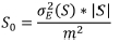
Here m is the mean of the target variable, S a block the size of the mesh, ISI its area, and oj(S) the extension variance of the variable, depending on its variogram. Then the ratio o²_E(S)/m² is the extension variance of the variable divided by its mean squared, which depends on the variogram of the variable divided by its mean.

The coefficient of variation of annual or quarterly Resources is given by

with S_pthe production area considered (annual or quarterly).

To link this method with the required rule of ±15% for annual or quarterly production volumes, the assumption is made that, at the level of Resources, the variable is Gaussian with mean m and variance o². Let Z be this variable, and Y=(Z-m)/o its associated standard Gaussian with standard cumulative density function G(). The probability p to be more than a certain deviation d from the mean can be written as p=P[Z-mI>dm], and so

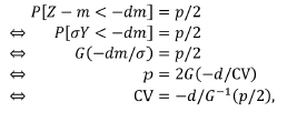
where the CV (coefficient of variation) is the ratio between the standard deviation and the mean: CV=o/m. With p equal to 10% and d equal to 15% (probability of 90% to deviate by less than 15%), the CV is 9.12%. A similar computation can be done for the lognormal case, resulting in a very similar CV value (9.19%), showing that the Gaussian assumption is not so important. In the following, the CV has been rounded to 9.2%.

Since the areas of a year of production and a quarter of production are linked, the CVs calculated over those two areas are linked too:

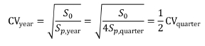
Therefore, in terms of category of Resources we have: For Measured Resources: CV_quarter <9.2°% and CV_year <4.6°% For Indicated Resources: CV_year <9.2% and CV_quarter <18.4%

 

Results

Coefficients of variation of the samples

Exploratory data analysis was done in two dimensions on the metal accumulations and thickness. For confidentiality reasons, the levels of the variables are not presented in this paper. Table II shows the values of the CV for the nickel and manganese oxide accumulations and thickness for the three layers.

 

 

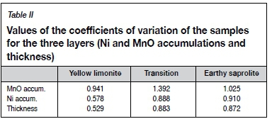
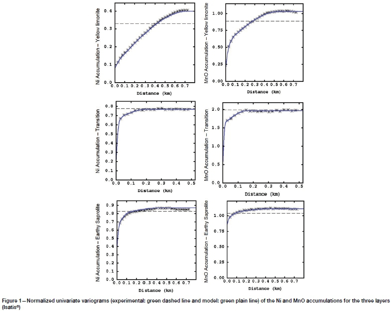
The yellow limonite layer presents the lowest coefficients of variation, and the transition and the earthy saprolite layers the highest. Altogether, the nickel accumulation and the thickness are less variable than the manganese oxide accumulation. The coefficients of variation for the nickel accumulation and the thickness are very similar: this is due the nickel grade being nearly constant within each layer. For this reason, results for those two variables are very close and only nickel accumulation is further displayed and commented on.

The experimental simple variograms and crossvariograms are calculated for each variable and each layer. These variograms were normalized by dividing each variable's values by its mean. As no anisotropy was observed on directional variograms up to several hundred metres, isotropy was assumed, and omnidirectional experimental variograms were computed. They are fitted with a nugget effect and spherical structures (up to four). Ranges and sills of the structures vary with the layer and the variable: nickel accumulation is more structured than the manganese oxide accumulation, while yellow limonite is highly continuous, unlike the transition zone and earthy saprolite (Figure 1).

Spatial continuity and structuration of the variograms are key points in the classification of Mineral Resources. As written in the CIM Definition and Standards (CIM, 2010): 'Mineralization may be classified as an Indicated Mineral Resource by the Qualified Person when the nature, quality, quantity and distribution of data are such as to allow confident interpretation of the geologicalframework and to reasonably assume the continuity of mineralization'.

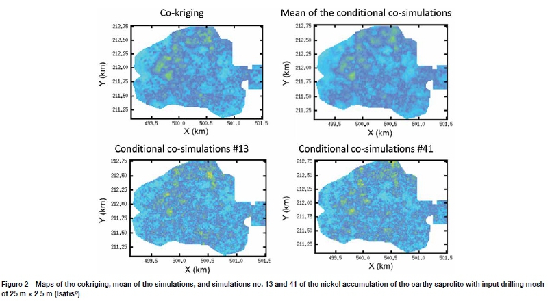
Visual display: maps of the cokriging and conditional cosimulations

Cokriging and conditional cosimulations are used conjointly to test the variability of the possible real values (simulated) around the predicted/planned (cokriged) values.

For the sake of visualization, four maps are displayed: cokriging, mean of the simulations, and two randomly chosen simulations (out of the fifty) of the nickel accumulation within the earthy saprolite. The input drilling mesh is 25 m χ 25 m. Cokriging and the mean of simulations are very close to each other, which is expected, although the mean of the simulations is a little bit smoother than the cokriging. The importance of shortest-range structural components is visible in the two simulations.

The legend is the same for the four maps: warm colours correspond to high nickel accumulation while cold colours indicate low nickel accumulation.

Conditional cosimulation results and comments

To test against the 15% rule, the results of the cokriging and the 50 conditional cosimulations were compared: if 90% of the cosimulations lie within ±15% of the cokriging, Mineral Resources are Measured or Indicated. Mineral Resources are classified as Measured if the comparison is done over an area equal to a quarter of year's production, and as Indicated if compared over an area equal to a year of production.

The 12.5 m χ 12.5 m block grid that contains the cokriging and the cosimulation results is coarsened to create bigger blocks whose areas are equal to a quarter or a year of production. The comparisons are done for each block.

Figures 3 to 12 are maps that show the probabilities that the cosimulation results are within ±15% of the cokriging results.

Yellow limonite

For a drilling mesh of 75 m χ 75 m, the results for blocks of a quarter of production are given in Figure 3.

For blocks of a year of production the results are given in Figure 4.

Although the grid mesh is about the same everywhere, one can see that the probability of deviating by less than 15% from cokriging is not the same for all blocks. This is likely due to the heterogeneity in the deposit, illustrated in Figure 2. To classify Mineral Resources, it was decided that if 50% of the blocks have a probability higher than 90%, then Mineral Resources are Measured (for blocks of a quarter of production) or Indicated (for blocks of a year of production). By applying this rule, it can be seen that a drilling mesh of 75 m χ 75 m is not sufficient to classify Resources as Measured (Figure 3) stricto sensu but is sufficient for Indicated (Figure 4), for both nickel and manganese oxide accumulations. However, for the nickel accumulation, 45% of the blocks have a probability greater than 90%, so that Mmineral Resources would be close to Measured with a drilling mesh of 75 m χ 75 m. This drilling mesh seems to be just above the limit between Measured and Indicated Resources with respect to nickel accumulation.

For a drilling mesh of 100 m χ 100 m, the results for blocks of a year of production are given in Figure 5.

For a drilling mesh of 125 m χ 125 m, the results for blocks of a year of production are given in Figure 6.

Following the same logic as presented earlier, a drilling mesh of 100 m χ 100 m is sufficient to demonstrate Indicated Mineral Resources in terms of nickel accumulation, but not in terms of manganese oxide accumulation, for which Mineral Resources would be Inferred (Figure 5). When the drill-holes are spaced at 125 m χ 125 m, Mineral Resources remain Indicated in terms of nickel accumulation (Figure 6).

Transition zone

For a drilling mesh at 25 m χ 25 m, the results for blocks of a quarter of a year's production are illustrated in Figure 7.

This drilling mesh is not sufficient to support Measured Mineral Resources for any of the variables of interest (Figure 7). However, it is sufficient to demonstrate Indicated Mineral Resources in terms of nickel accumulation (Figure 8). For manganese oxide accumulation, Mineral Resources are Inferred.

A drilling mesh of 50 m χ 50 m (Figure 9) is just sufficient to demonstrate Indicated Mineral Resources in terms of nickel accumulation and seems to mark the limit between Indicated and Inferred. For the manganese oxide accumulation, Mineral Resources are Inferred.

Earthy saprolite

For the earthy saprolite, the same maps can be drawn and the following can be concluded (Figures 10, 11, and 12).

> A drilling mesh of 25 m χ 25 m is insufficient to demonstrate Measured Mineral Resources for any of the variables (Figure 10). However, in terms of nickel and manganese oxide accumulations it is adequate to support Indicated Mineral Resources (Figure 11).

> A drilling mesh of 50 m χ 50 m is insufficient to demonstrate Indicated Mineral Resources for any of the variables: Mineral Resources are Inferred (Figure 12).

In all the above examples, the probability of the conditional simulations deviating by less than ±15% is not constant throughout the deposit: some areas are more variable than others, and those areas differ from one variable to another. Conditional simulation is a powerful tool for the geologist to identify areas that require denser drilling in order to increase confidence in the chemistry of the deposit (and subsequently the chemistry of the ore fed to the plant) and to link those areas with the geology and the mineralogy.

Specific areas method: results and comments

The efficiency of the drilling mesh has been tested through the calculation of the specific areas method: the lower the specific area, the more efficient the drilling mesh. Results are displayed in Table III for all the drilling meshes tested, for the nickel (Ni) and manganese oxide (MnO) accumulations in each of the three layers.

The results are similar to the previous observations: for the same drilling mesh, specific areas for the yellow limonite are lower and thus the mesh is more efficient due to the high geological continuity of this layer.

Attention is drawn to the difference between the nickel accumulation and the manganese oxide accumulation, the latter being less continuous in each of the three layers.

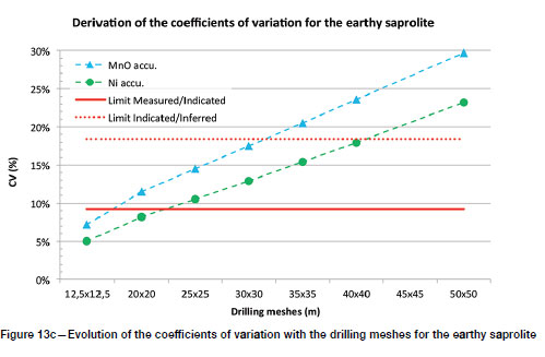
Calculations were not done for drilling meshes greater than 50 m χ 50 m for transition zone and earthy saprolite because these lie in the category of Inferred Mineral Resources (see Figure 13c).

 

 

 

 

 

 

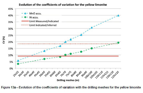
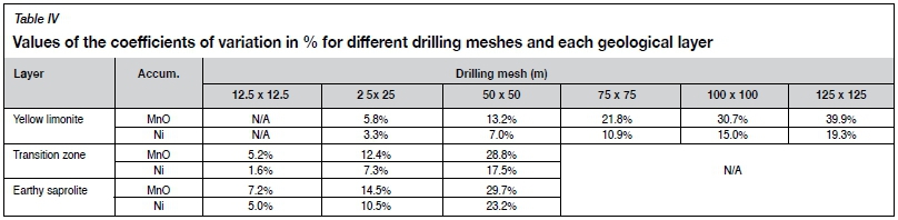
A graph of coefficients of variation against drilling mesh for a quarterly production area is drawn in Figure 13, with selected values shown in Table IV.

Differences between nickel and manganese oxide accumulations are obvious: while Mineral Resources are Measured until 65 m χ 65 m for nickel, they are Measured only up to 35 m χ 35 m for manganese oxide (Figure 13a). This gap persists for Indicated Mineral Resources, where a drilling mesh of 120 m χ 120 m marks the limit between Indicated and Inferred for nickel accumulation, this limit being 70 m χ 70 m for manganese oxide accumulation.

For the nickel accumulation, the limit between Measured and Indicated classifications appears to be very similar for simulations and specific areas (compare Figures 4 and 13a: 75 m χ 75 m is not quite sufficient for Measured in both cases). The mesh separating Indicated from Inferred categories is slightly smaller for specific areas (120 m χ 120 m for nickel accumulation, while simulations demonstrate Indicated for 125 m χ 125 m spacing; 70 m χ 70 m for manganese oxide accumulation while simulations give Indicated for 75 m χ 75 m spacing).

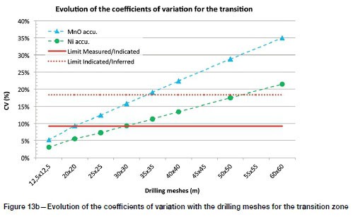
Similar differences between nickel and manganese oxide accumulations are observed for the transition layer (Figure 13b). For this layer, drilling meshes that mark the limits between Measured and Indicated are much denser than for the yellow limonite: 30 m χ 30m for Measured/Indicated and 50 m χ 50m for Indicated/Inferred, when considering the nickel accumulation. Recall that the limit between Indicated and Inferred at 50 m χ 50 m is the same as the one observed with the conditional simulations. These limits are reduced to 20 m χ 20 m and 35 m χ 35 m respectively for manganese oxide accumulation.

For the earthy saprolite, drill spacing limits are a bit smaller but close to those of the transition layer, with a drilling mesh between 20 m χ 20 m and 25 m χ 25 m for the limits of Measured/Indicated, and 40 m χ 40 m for the limits of Indicated/ Inferred, when considering nickel accumulation (Figure 13c). These limits are reduced to 1 6 m χ 16 m and 32 m χ 32 m respectively (approximately) for manganese oxide accumulation.

As shown in the 'Methods' section, there is a direct link between the coefficients of variation and the probability of having a deviation of ±15%. In terms of probability a clear interpretation of the relationship between drilling mesh and category of Mineral Resources is provided (Figure 14).

The coefficients of variation and the probability curves confirm the high continuity of the yellow limonite compared with the two other layers. The manganese oxide accumulation is less continuous than the nickel accumulation for all three layers.

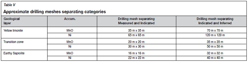
From the graphs in Figures 13 or 14 the approximate drilling meshes separating the different categories of resources can be deduced (Table V).

Recall that the coefficients of variation calculated with the specific areas method depend on three major factors: the spatial continuity (i.e. the variogram model), the drilling mesh, and the production area. The following section aims at showing the influence of these factors.

Specific areas method: Influence of the variography

To quantify the influence of the variography only and remove the effect of the production areas, similar calculations are done using the same production area outline for all the three layers, here the actual production area of the yellow limonite. The evolution of the coefficients of variation with the drilling meshes is displayed in Figure 15 for nickel accumulation.

Using equivalent production areas highlights the effect of the spatial variability: the yellow limonite is more continuous than the other layers, and the transition and earthy saprolite layers have similar results, they are both very discontinuous (and also have similar variogram models). On the other hand, the effect of the production area is important: the production area of the earthy saprolite is half that of the two other layers and there is a greater impact on the coefficients of variation (about 1.4 times larger when taking its production area).

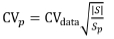
To test the reliability of the coefficients of variation, the coefficients of variation for production areas have been recalculated using pure nugget effect variograms, with a nugget value equal to the variance of the sample data. Denoting the CV of the sample data by CV_data and the CV of the production area by CV_p, the specific area becomes

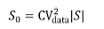
so that

The results of the coefficients of variation calculated over an area equivalent to a quarter of a year's production (actual for each layer) are summarized in Table VI.

For the transition zone and the earthy saprolite, the coefficients of variation are a bit higher than those listed in Table IV. In fact, the variograms for those layers have a high proportion of nugget effect.

For the yellow limonite, however, CV results using a pure nugget effect are much higher than the ones calculated previously: the yellow limonite is much more structured, and the proportion of the nugget effect is significantly lower. However, it is unlikely that even with a coarse exploration drilling pattern it would be impossible to miss the structures as the layer is highly continuous.

Overall, the results are consistent and in the same order of magnitude. When a structure exists but the resolution of drillhole spacing is not fine enough to characterize it, the CV results using pure nugget effect are a bit pessimistic (i.e. too high) as the structure is unknown. Even if the spatial variability is not perfectly known (as in the exploration phase), the specific areas method can still be used to classify Mineral Resources.

 

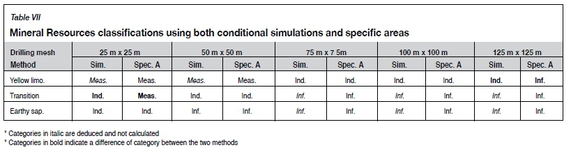
Mineral Resources classification

Based on the nickel accumulation results, the following Mineral Resources classification is proposed, and a comparison between results using the simulations or the specific areas method can be made. Table VII displays these results.

The classification differs between the two methods for transition zone at 25 m χ 25 m and yellow limonite at 125 m χ 125 m: in both cases results for the specific areas method are very close to the limit between one category of Mineral Resources and the following one. The two methods in general yield similar results, and the differences are minor. If one category is to be selected, the conditional simulations give the most accurate results and can help in choosing between one result or another.

 

Comments and perspectives

This study allows a comparison of two geostatistical methods for classifying Mineral Resources from the point of view of the drilling mesh. Both methods yield almost the same results, and it can be concluded that the specific areas method is a valid method to classify resources. However, they differ in their purposes as they do not share the same benefits and limitations (Table VIII).

 

 

The drilling mesh used as input is a limiting factor for the direct use of conditional simulations as only meshes that are a multiple of the existing mesh can be tested. Testing a refined mesh (or any other mesh) from a currently available mesh can be done by using a less direct method: first, simulating values on the refined mesh conditionally on the available one, and then simulating values everywhere else conditionally on the refined mesh (Geovariances, 2018). A similar procedure can be done starting from a nonconditional simulation, but this would ignore the possible heterogeneity of the deposit.

Both methods could be used together in any two-dimensional deposit: the specific areas method as a routine to obtain a good order of magnitude and define the drilling meshes that mark the limits between categories of Mineral Resources, and conditional simulations to validate those limits.

Conditional simulations can also be very useful to define areas that require denser drilling to refine the understanding where elements are more variable.

The classification presented in this paper only takes into account the nickel accumulation. Both methods could be extended to other auxiliary variables, such as the manganese oxide that plays an important role in the nickel recovery process. A classification based on this auxiliary variable only would be much more restrictive. However, classification would then become a multivariate issue that considers all the elements that are important in the process of recovering nickel.

For classification using conditional simulations, Dohm (2005) proposed considering 'units representing likely production periods'. In the case presented, the production areas were represented by simple squares. As noted by Rossi and Deutsch (2014), such a simple and current choice may be a significant limitation, as the actual production may come from different areas of the mine. It must therefore be recognized as a convenient simplification. While it would be possible to consider other shapes for the production areas when using conditional simulations, such a consideration does not exist when using the specific areas method. Instead, the production area is then considered as a union of blocks having the size of the mesh, wherever they are (Rivoirard and Renard, 2016) and this makes the calculations simple. Note that the specific area itself, expressed in m², can be used to measure and compare the efficiency of a grid, irrespective of any production.

Another simplification was made by working in two dimensions for each layer. This implicitly assumes that, during each production period considered, each layer is exploited from top to bottom where it is mined. Considering a finer exploitation would require working in three dimensions. The specific areas method also is applicable in three dimensions: the specific area in m² is replaced by a specific volume in m³, which measures the efficiency of the three-dimensional sampling design. Both methods are also applicable with an irregular sampling pattern.

 

Acknowledgements

The present work was performed when the first author, previously Geology Superintendent at Vale New Caledonia, was undertaking the CFSG Master (Cycle de Formation Spécialisée en Géostatistique) at MINES ParisTech, Fontainebleau, France. For their guidance, the data provided, and the efforts they made to make this Master of Geostatistics happen, the author would like to thank the technical team of Vale in Canada and in New Caledonia, namely Tim R. Lloyd, Principal Resource Geologist (retired), Chris Davis, Head of Geology and Mine Design, Jerome Dufayard, Geology and Mine Planning Manager, and Benoit Laz, Geologist.

 

References

Canadian Institute of Mining, Metallurgy and Petroleum. 2011. National Instrument 43-101 - Standards of Disclosure for Mineral Projects. Westmount, Quebec, Canada.         [ Links ]

Canadian Institute of Mining, Metallurgy and Petroleum. 2010. CIM Definitions Standards - For Mineral Resources and Mineral Reserves. 10 pp. http://web.cim.org/UserFiles/File/CIM_DEFINITON_STANDARDS_Nov_2010.pdf        [ Links ]

Chiles, J-P. and Delfiner, P. 2012. Geostatistics: Modeling Spatial Uncertainty. 2nd edn. Wiley, New York.         [ Links ]

Dohm, C. 2005. Quantifiable mineral resource classification - A logical approach. Proceedings of Geostatistics Banff2004, vol. 1. Leuangthong, O. and Deutsch, C.V. (eds.). Kluwer Academic, Dordrecht. pp. 333-342.         [ Links ]

Geovariances. 2018. Testimonials & Success Stories. Conditional simulations improve confidence in mineral resource classification. https://www.geovariances.com/en/testimonials/conditional-simulations-imporve-confidence-in-mineral-resources-classification        [ Links ]

Geovariances. 2017, Isatis software. https://www.geovariances.com/en/software/isatis-geostatistics-software        [ Links ]

Rivoirard, J. and Renard, D. 2016. A specific volume to measure the spatial sampling of deposits. Mathematical Geosciences, vol. 48. pp. 791-809.         [ Links ]

Rivoirard, J., Renard, d., Celhay, f., Benado, d., Queiroz, C., Oliveira, L-J., and Ribeiro, D. 2016. From the spatial sampling of a deposit to mineral resources classification. Quantitative Geology and Geostatistics. Proceedings of Geostatistics Valencia2016, vol. 19. Gomez-Hernandez, J.J., Rodrigo-Ilarri, J., Rodrigo-Clavero, M.E., Cassiraga, E., and Vargas-Guzmán, J.A. (eds.). Springer, Dordrecht.         [ Links ]

Rossi, M.E. and Deutsch, C.V. 2014. Mineral Resource Estimation. Springer, Dordrecht. 332 pp.         [ Links ] ♦

 

 

Correspondence:
F. Isatelle
isatelle@geovariances.com

Received: 7 Mar. 2019
Revised: 28 Jun. 2019
Accepted: 30 Jun. 2019
Published: October 2019