GENERAL PAPERS

 

Coupling simulation model between mine ventilation network and gob flow field

 

 

F-l Wu^I; Y. Luo^II; X-t Chang^I

^ICollege of Safety Science and Engineering, Xi'an University of Science and Technology, China
^IIDepartment of Mining Engineering, West Virginia University, USA

Correspondence

 

 

---

SYNOPSIS

Many numerical simulation studies of coal spontaneous combustion have focused on the leakage flow field in the mine gob. However, most of these studies isolate the gob from the mine ventilation system, failing to consider the effects of air leakage on gob boundary conditions. A novel model coupling the mine ventilation network (MVN) and gob flow field (GFF) has been developed to simulate the overall mine ventilation system. The concept of network boundary node was proposed and the corresponding air flow rate balance equations were developed based on the node pressure method for MVN calculation and the finite element method for GFF simulation. These equations, containing the rate of air flow not only from the branches but also from the gob, revealed the coupling relationship between 1D MVN and 2D/3D GFF. An iterative solution technique was developed to solve the coupling model, which has been incorporated into a program i-MVS. An illustrative example with coarse mesh is used to verify the stability and convergence of the model. Results of an application case show that the coupling model has sufficient precision and the developed software is efficient in implementing the computations.

Keywords: gob flow field, mine ventilation network, spontaneous combustion, longwall mining, numerical simulation.

---

 

 

Introduction

Ideally, air leakage into mine gob is not desirable for underground coal mines employing a bleederless ventilation system. Such air leakage, an unavoidable phenomenon, is the major cause of spontaneous combustion - a serious concern for coal mine safety due to the high risk of it causing severe mine fires and even explosions (Ozdogan et al., 2018). Approximately 17% of the 87 reported fires in underground coal mines in the USA from 1990 to 1999 were caused by spontaneous combustion (Yuan and Smith, 2008). More than 60% of underground fires in China started from spontaneous combustion in gobs (Xia et al., 2016).

A good understanding of the gob flow field (GFF) is helpful for developing strategies to control and prevent spontaneous combustion and explosive methane concentration at the tailgate T-junction - both of which are of great concerns for mine safety. It should be noted that controlling spontaneous combustion in the gob and the explosive methane concentration at the tailgate T-junction require different ventilation approaches. One of the best ways to identify the gob zone prone to spontaneous combustion is simply to analyse the ventilation flow in the gob. Spontaneous combustion could occur in a zone where the heat generated by the low-temperature oxidation of coal is inadequately dissipated by conduction or convection in the coal incubation period, which can be tested in the laboratory (Yang et al., 2014). Once this zone is delineated, a minimum longwall retreating rate can be determined so that the life of the zone can be kept less than the incubation period for spontaneous combustion (Tripathi, 2008). Based on past research, an air velocity range of 0.0017-0.004 m/s in the gob has been commonly used to delineate the combustion-prone zone because the higher air velocity can carry heat away quickly while a lower air velocity would not provide sufficient oxygen for the self-heating process (Wang, 2009; Shao, Jiang, and Wang, 2011). However, due to the inaccessibility of the gob area it is nearly impossible to make a direct observation or measurement of the gob air flow. Therefore, accurately simulating the GFF remains an important research topic in the area of mine ventilation and safety in underground coal mines.

Many numerical studies have been conducted to simulate the GFF in order to understand the mechanisms of spontaneous combustion. Saghafi, Bainbridge, and Carras (1995) and Saghafi and Carras (1997) performed numerical modelling of spontaneous combustion in underground coal mines with a U-ventilation system. Yuan and Smith (2008) numerically modelled spontaneous combustion for a bleeder ventilation system with two gobs using the commercial CFD program FLUENT. Xia, Xu, and Wang (2017) developed a coupled two-dimensional numerical model to study the flow behaviour of gas in the gob area by applying a developed software package and the commercial CFD program COMSOL. However, these research works basically isolated the gob from the mine ventilation system, with only predefined boundary conditions. The computational domain mainly included the gob area, failing to consider how the boundary conditions are affected by the air leakage. In fact, the simulation results for GFF readily vary with the prescribed boundary conditions. Additionally, any changes in the mine ventilation system can change the boundary conditions of GFF and vice versa. The predefined static boundary conditions have to be changed manually in the gob field model to reflect such changes. If the boundary conditions can be simulated simultaneously, it will allow the simulation of complex boundary conditions for GFF. However, little modeling work has adequately considered the incorporation of cross-coupled boundary conditions between the mine ventilation system and GFF.

The integration of the mine ventilation network (MVN) and GFF offers the capability of considering the complex boundary conditions. In the past decades many MVN programs with a 1D model have been developed for simulating the air flow or fires only in underground mine airways; for instance, MFIRE, VentSim, VnetPC, and VentGraph (Zhou and Smith, 2011; Zhou, Smith, and Yuan, 2016). Such programs have become an essential tool for mine ventilation design and routine ventilation management. Based on an MVN program an early model (Brunner, 1985) divided the gob into many airways to simulate the effects of significant gob air leakage on network analysis. However, using airways to denote the gob flow is not precise enough to compare with CFD technology. A more recent study (Wedding, 2014) incorporated a network model into a commercial CFD program, which in some degree created a simple integration between the network and gob. Wedding's research shows that it is still a very challenging task to couple a 1D network flow model and the 2D/3D field flow model for realistic simulation in mine ventilation. In this current research, the mine ventilation system is treated as being entirety composed of the MVN and GFF, and a novel coupling model is developed and then implemented in a computer program for mine ventilation simulation.

 

Ventilation network analysis based on nodal pressure

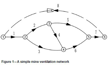
A mine ventilation system consisting of various arrangements of airways can be depicted as a connected and directed graph in which network branches are connected at nodes. As an example, a greatly simplified MVN containing eight branches and six nodes is shown in Figure 1. Network analysis has been used routinely in mine ventilation planning to distribute the required air flows to various working faces.

 

 

The ventilation network analysis applied in this paper is based on the nodal pressure method, in which the nodal pressures are taken as the unknowns. In a given network with m nodes, take any node as a base node and its pressure is set to zero; the pressures at the remaining m-1 nodes are relative to the base node pressure. In addition, according to Kirchhoffs first law, the total quantity of air leaving a node must be equal to that entering this node. The governing equations of an MVN can be established by the air flow balance equation at each of the rest (m-1) of the nodes (Hartman et al., 1997).

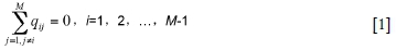
In Equation [1], q_tJis the air flow rate in the branch connecting the nodes i andj. The flow rate q_tJis set to positive when air leaves node i and to negative when air enters the node. There are three types of branches. The first type is a general branch, and by the Atkinson equation (Hartman et al., 1997) q_iJ can be expressed as:

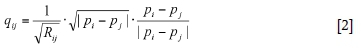
where p_iand P_jrepresent the pressures at nodes i and j based on the zero pressure node, and Rj is the resistance of the branch connecting nodes i andj, in units of Ns²/m⁸. The second type is a fan branch between nodes i and j where a fan is placed, such as branch 8 in Figure 1, and

In Equation [3] F_g(H) is the characteristic curve function of the fan, and H is the fan's pressure in units of Pa. Since F_g(H) is always positive, coefficient b_ijis used to represent the flow direction related to node i, and b_ij equals +1 when air is leaving node i and -1 when it is entering node i. The third type is the fixed quantity branch, which means the air flow rate is set to a fixed value under any circumstances, so

In Equation [4] Qj is a positive constant air flow rate in the branch connecting nodes i andj. When the expressions for all three types of branch are substituted in Equation [1], only p_i (i = 1, 2,..., M-1) are unknowns. Because of the nonlinear nature of Equation [1], Newton's method is used to solve the equations in this study (Wu et al., 2016).

 

Gob flow field model based on the finite element method

Steady linear seepage model

The mine gob is the area where coal has been mined and the space is filled with caved rock (Karacan, 2009). A typical gob of a longwall panel with a bleederless U-ventilation system is shown in Figure 2. The GFF is caused by the air leaking from the working face to the gob. The air flow in the gob can be firstly assumed to be an isotropic steady linear seepage flow which obeys the Darcy Law and the continuity equation, which can be expressed in the following two differential equations in a Cartesian coordinate system:

 

 

 

where V is the seepage velocity in the gob in m/s; T is the hydraulic conductivity in m/s; V is the Hamilton operator - in 2D space and it can be expanded into 3D space; P is the pressure at any point in the gob and is also expressed in relative pressure. By substituting Equation [5] into Equation [6], the mathematical model of seepage flow can be expressed as the following differential equations:

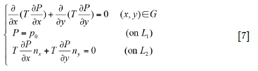
In Equation [7], G is the domain of the gob area; p₀ represents the known pressures along L₁, which is the boundary with air leakage (the method used to determine the pressures will be discussed later); n_x, n_yrepresent the components of the outer unit normal vector of L₂, which are the boundaries of no air leakage.

The purpose of applying the finite element method for Equation [7] is to obtain the pressure function of P(x, y), which is represented by a series of interpolating functions. To do this, the surface G is divided into a sufficient number of triangular elements and nodes as shown in the expanded drawing in Figure 2. The pressure interpolating function Ρ_Δ (x, y) for each element can be expressed as

In Equation [8], p'_i, pj, and p _kare pressures at the triangular element nodes which are numbered in counterclockwise around the triangle; N_;, Nj, N_kare shape functions which only have relations to the coordinates of each element and can be described as N = 0.5(α+>χ+<^)/Α_Δ, Nj = 0.5(¾. + bjX+Ojf) )Μ_Δ, N_k= 0.5(a_k + b_kx + c_ky) )/Α_Δ, where Α_Δis the area of each triangular element in units of m². The coefficients a, b, c can be determined from the coordinates of each triangular element, which are: a_t= Xjyk-Xkyj, b = yj -y_k, c = Xk - χ, a = x_ky_{- xj_k, bj = yk -y, Cj = χ - xk, a_k= xy - x^y, b_k= y; -y, c_k= xj - If every node pressure can be determined, the function of P(x, y) on the entire gob can be represented by all of the interpolating functions of Ρ_Δ (x, y).

It has been proven that Equation [7] is the same as the functional of Equation.[9], meaning that the solution of Equation [7] makes I(P) taking the extremum value.

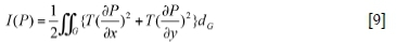
Now Δ is used to represent the surface of one element, then

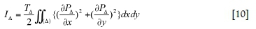
where Τ_Δrepresents the hydraulic conductivity of each triangular element and can be calculated by the method proposed in the next section. By numerical integration, I(P) in Equation [9] can also be calculated as:

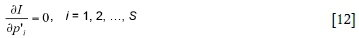
where Σ_Δ is a summation operation to all of the elements. When Equation [8] and Equation [10] are substituted into Equation [11], I(P) becomes a multivariate function I(p\,p'₂,...,p'_s) instead of a functional formula, where S is the counts of gob nodes not on the boundary L₁. To get the extremum value of I(p ₁, p'₂,..., p'_s), equations can be obtained:

Substituting Equation [8] and Equation [11] into this equation yields

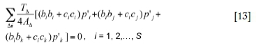
where Σ is a summation operation of all elements which are connected with node . The pressure values of gob nodes on L₁ also appear in Equation [13], but as known values. Equation [13], a linear system of equations aboutp ₁ (i = 1, 2,..., S), is the governing equation of the steady linear seepage model in the gob.

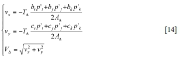
When all gob node pressures are solved using Equation [13], the air flow velocity ν_Δin each element and its components of v_x and v_ycan be calculated by:

 

Distribution of hydraulic conductivity and porosity of gob

Research has shown that the hydraulic conductivity or porosity in gob generally meets the characteristic of the O-ring distribution (Xia, Xu, and Wang, 2017; Zhang, Tu, and Zhang, 2016). It can be estimated using the following empirical equations:

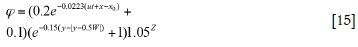
where x, y are the coordinates of a given point in the gob as shown in Figure 2, where the X axis of the coordinate system is along the intake entry and the Y axis is along the longwall face; x₀ is the distance from the cut-open position to the Y axis; u is the advance rate; t is the advance time; φ is porosity; W is the width of the gob; E is gob permeability; d is average particle size; υ is the kinematic coefficient of viscosity of air; g is the acceleration due to gravity. For a 2D model, Z equals zero.

Nonlinear seepage model

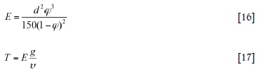
The seepage field of air flow in the gob, especially in the area adjacent to the longwall face, is nonlinear and obeys the Bachmat equation (Bear, 1972):

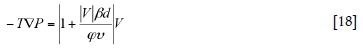
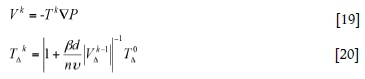
where β is a dimensionless particle shape coefficient of the medium. An iterative solution technique based on the linear seepage model can be applied to solve the nonlinear seepage model (Li, Liu, and Wu, 2008). The iteration equations [19]) and [20] can be deduced from Equation [18] and the iteration flow chart is shown in Figure 3.

 

 

 

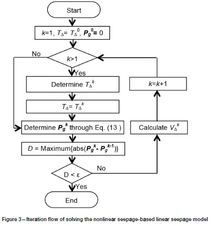
It should be noted that Equation [19] still keeps the form of Darcy's Law in Equation [5], meaning that V/ of each element can be evaluated using the linear model of Equations [13] and [14] in which Γ_Δ equals T/. The term T_A^kis the k^th correction value for the original Γ_Δ⁰ value determined using the method in the previous section for each element. Equations [19] and [20] indicate that the nonlinear seepage in gob can be treated by Darcy's Law but with a set of hydraulic conductivities corrected by a velocity-dependent factor. In Figure 3 all the operations about Γ_Δ⁰, T_A^k, V/ are for each element; P_g^kis a vector of the gob node pressures determined in the k^thiteration by solving Equation [13]; D is the maximum absolute value of the difference between P_g^kand P_g^k-1. The iteration exits until D is less than a preset tolerance, ε.

 

The coupling model between MVN and GFF

Boundary coupling model between the longwall face and gob

The previous sections have shown that distributions of air pressure from MVN simulation can be used to describe the boundary conditions for the gob simulation model. By combining the 1D ventilation network model with a 2D or 3D flow field model, a novel approach to simulate air flow along the longwall face and inside the longwall gob is developed. The representation of the longwall face and its gob (Figure 2) is shown in Figure 4.

 

 

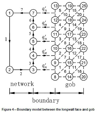
In Figure 4, the solid lines represent network branches and triangular shapes with dashed edges represent the gob elements. The elements adjacent to the longwall face (numbered 1 to 5) are called boundary elements. The branches (3 to 6) representing the longwall face area are connected between nodes 3 and 7. The nodes numbered from 3 to 7 are called the network boundary nodes. As shown in Figure 4, the five boundary elements require five network boundary nodes. Branch 1 represents the remaining part of the mine ventilation network, which often contains hundreds of branches in a real model. The dashed lines with arrows are treated as virtual branches which represent the flows between the gob and working face. For GFF, the pressures at nodes 8-13 on the boundary L1 can be set through network boundary nodes, i.e. the pressure at node 8 should be equal to that at node 3 and the pressure at node 9 should be equal to the average pressure at nodes 3 and 4. On each virtual branch p y is the rate of air flow between boundary elementj and node i, and can be calculated by the results of GFF:

where Aj is the side face area of boundary elementj'; n_jx, ny are the components of the unit vector in the direction of the outer normal of the boundary edge of elementj'; v_Jx, V_jyare components of air flow velocity of element j and can be calculated from Equation [14]. The value of p y resulting from Equation [21] is positive for air leaving element j and entering node i, otherwise it is negative. So when p y is considered in the air flow balance equation at each network node, Equation [1] can be rewritten as

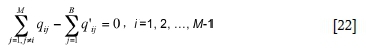
where B is the number of boundary elements on L₁. Equations [21] and [22] show that MVN simulation results depend heavily on GFF simulation outputs, while Equation [13] shows the MVN results are necessary for the boundary conditions of GFF simulation. Therefore, p y is the coupling linkage between the MVN and GFF models.

The flow chart for the iterative solution process for determining air flows using the proposed coupling model is shown in Figure 5. For the purpose of comparison, a non-coupling model that is currently the common practice in GFF simulation is illustrated in Figure 5. In the non-coupling model, MVN simulation is performed only once and the results are applied to the subsequent GFF simulation. In Figure 5, Q_g^kis a vector of p j calculated in the k^th iteration and D is the maximum absolute value of the difference between Q_g^kand Q_g^k-1. In the coupling iterations, the MVN simulation begins with Q_g° = 0, and then the gob simulation runs with the boundary node pressures determined from the network boundary nodes. In the following network simulation each Q_g^kwill have a set of values as a fixed quantity branch added into each network boundary node. The iteration does not stop until D is less than the preset tolerance ε. If the gob area and the longwall face branch are divided into a sufficient number of elements and fine branches, the coupling model can adequately approximate the reality of air flow in the longwall face and the gob.

 

 

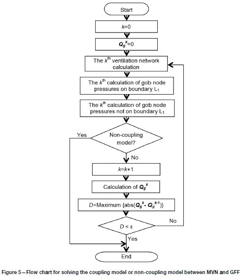
Therefore, using the proposed coupling model between the MVN and GFF, all of the nodal pressures can be determined by solving the governing equations [13] and [22] using the iterative solution process as depicted in the flow chart in Figure 5.

Software development and demonstration example

An integrated mine ventilation simulator (i-MVS) program with a visual interface was developed to encapsulate the coupling model with 2D gob in VC++ and ObjectARX (Yang et al., 2014). Through i-MVS the finite element meshing and ventilation network modelling can be accomplished.

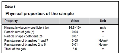
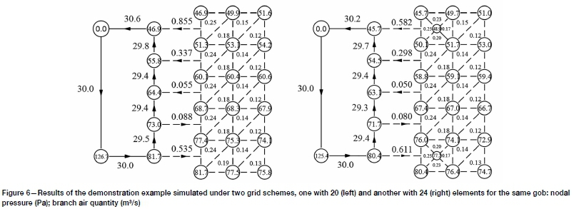
In order to validate the proposed model and developed computer program, especially in mathematics, the simple example shown in Figure 4 is used for demonstration purposes. Coarse triangular elements with 60 m sides are used to represent the longwall gob so that simulation results for the elements and branches can be presented and checked easily. The air flow of the fixed quantity (branch 1) is set to 30 m³/s while the other input parameters for the simulation are listed in Table I. The simulation is conducted using the developed software with zero preset pressure at node 1. In this example, the iterative process shown in Figure 5 converges to ε=10^-5 after five iterations.

 

 

The simulation results are shown in the left-hand graph of Figure 6, where the porosity is shown in triangles; the nodal pressure in circles; the air quantity in the network is labelled beside the branch. It shows that air leaks into the longwall gob in the first half-length of the longwall face while the leaked air returns to the longwall face in the second half of the face, an important result that cannot be realized by using a 1D MVN solution alone.

Like other discretized numerical simulation methods, the finite element method also provides an approximation solution. As described previously, once the physical properties of porosity, velocity, etc. for each element are specified, the accuracy of the solution depends how the domain of the study is discretized. Only when sufficient elements are used can the solutions approach the reality (Zienkiewicz, Taylor, and Zhu, 2015). Another similar classic example in CFD is that the coarse mesh used to simulate the convection-diffusion model always causes an oscillation (Heinrich et al, 1977; Zienkiewicz, Taylor, and Nithiarasu, 2014). However, the solution obtained by rough grids certainly conforms to the governing equations. As in this example, all nodes are in accordance with the flow balance equation, except node 1 where an imbalance in air flow of 0.6 m³/s is observed since the equation about node 1 is not in the governing equations as shown in Equation [1]. This imbalance of 0.6 m³/s is the difference between the rate of air flow entering and that leaving the gob. The right-hand graph of Figure 6 shows that the imbalance is reduced to 0.2 m³/s when two elements are added into the two corners near the face. The total influxes to the gob in the two solutions are 0.623 m³/s and 0.691 m³/s, and the corresponding errors reflected by imbalance are about 96.3% and 28.9%, respectively. Therefore, this imbalance is indeed caused by the coarse mesh used. The two solutions of the example show that the proposed mathematical model is valid and the iterative control equation for the solution process is steady and converging. Finer meshing used for the gob could eventually reduce the imbalance problem to an insignificant level.

 

Software application

Numerical case and simulated conditions

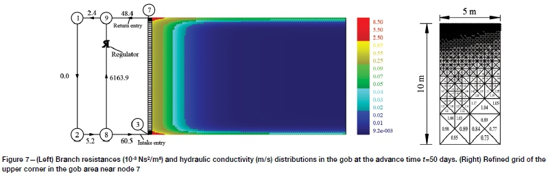
A realistic longwall panel with a U-ventilation system is adopted in the numerical simulation model. The coupling model of the case is shown in Figure 7. The panel is 2500 m long, 300 m wide, and 6 m high from the bottom of the coal seam. With an advance rate of 10 m/d, the active gob is 500 m long when the advance time is 50 days. This ventilation scheme and the panel dimensions are typical of longwall operations in the northern region of Shaanxi Province, China. The program provides the functions of meshing and automatic refining for the gob area. Firstly, the gob was divided into isosceles right triangular elements with 5 m edge length by using a structured grid generation method like that used for the left-hand graph of Figure 6. The principle of mesh refinement is to make the difference between the hydraulic conductivities of any two adjacent elements not exceed a preset small value, 0.2 m/s in this case. In the left-hand graph of Figure 7, the gob area is totally meshed into 19 368 elements and the longwall face is divided into115 fine branches accordingly. Finer meshes are automatically generated in the two gob corners where most of the air flow enters and leaves the gob, in order to gain an accurate simulation of air flow in those areas since the porosity varies greatly in these places as described in Equation [15]. The right-hand graph of Figure 7 shows the mesh refinement effect over an area of 5 m depth and 10 m width at the upper corner of the gob, where the hydraulic conductivities are shown in triangles. In the left-hand graph the branch resistances are beside the lines and the gob is colour-coded with non-uniform hydraulic conductivities. The flow rate of the fixed quantity branch connecting nodes 1 and 2 is set to 35 m³/s. In a typical Chinese longwall panel, an entry connecting the intake and return entries is placed at the panel recovery end for various production and safety purposes. A ventilation regulator, in the form of an adjustable door, is installed at this connecting entry to control the air flow to the longwall face (typically 30 m³/s), and that flows through the connecting entry as show in the left-hand graph of Figure 7. The resistance of the longwall face per 100 m is 0.02083 Ns²/m⁸ and the other physical properties are the same as in the previous section. With a parallel computational method (Schenk and Gärtner, 2004) adopted in the software, only several minutes of computation time was added for this complicated simulation.

Analysis of results

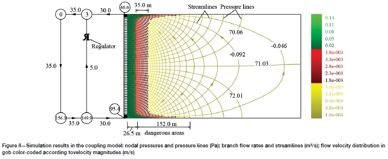
The simulation results are shown in Figure 8. In the network, the nodal pressure is shown in the circle and air quantity is beside the branch. The pressure distribution in the gob area is plotted as 50 contour lines with a pressure drop interval of 0.98 Pa. The distribution of air flux is also plotted in contour form (streamline with arrow) with an interval of 0.046 m³/s. These lines are colour-coded according to velocity. Red is used to highlight the zone prone to spontaneous combustion where the air velocity ranges from 0.0017 to 0.004 m/s. For this simulation case, the width of this zone varied between 35 m and 152.0 m. Figure 8 shows that the further away from the longwall face, the less the air leakage as indicated by the lower velocity. The combustion-prone zone is always some distance behind the longwall face, as marked by the green colour. The red zone, representing the gob area with higher spontaneous combustion risk, is wider near the panel edges along the panel longitudinal direction. Therefore, an appropriate longwall retreating rate should be determined using the width of the combustion-prone zone near the panel edges in order to prevent spontaneous combustion.

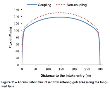
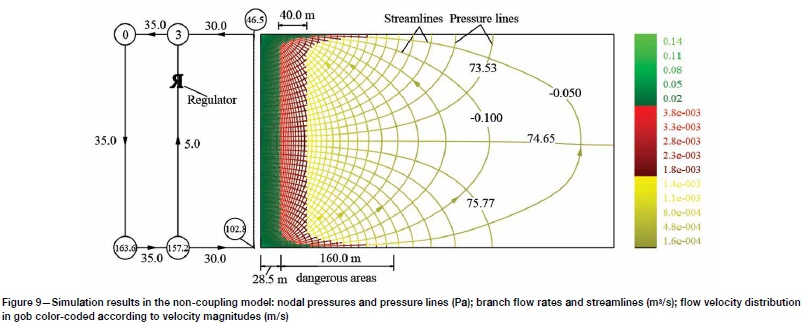
For the purpose of comparison, a non-coupling simulation as descripted in Figure 5 was conducted. The result of the non-coupling model is shown in Figure 9. The profiles of relative pressure and leakage flux along the longwall face from the two models are shown in Figures 10 and 11, respectively. Inspection of both simulation results shows that most of the air leakage in and out of the gob occurs at the intake and return corners, as shown in Figure 11. The total leakages from the coupling and non-coupling models are 138.2 m³/min and 150.7 m³/min, respectively. The differences between the rate of air flow entering and that leaving the gob in the coupling and non-coupling models are 0.031 m³/s and 0.035 m³/s, and the corresponding errors reflected by the imbalances are 1.3% and 1.2%, respectively. This is so insignificant that it is difficult to see the differences in Figures 8, 9, and 11. Therefore, refining the meshes of the gob can greatly reduce the flow imbalance problem encountered in demonstration case 1 (Figure 6).

 

 

 

 

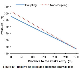
In general it is the fan that drives air flow in the airways and gobs. In a local gob area, there is always a pressure difference along the streamline, as shown in Figures 8 and 9, which drives air to flow in the gob. Meanwhile, the GFF is determined by its pressure boundary condition, which is determined by the distribution of the air pressure drops along the longwall face as descripted previously. The total pressure drops along the longwall face also shows how much energy is used to drive the air flow through the longwall face and gob area. Therefore, the pressure distributions along the longwall face in the two models are the focus of comparative analysis.

Comparison of the results in the two models shows that air leakage has an obvious influence on the boundary conditions of the GFF. Figure 10 shows that the air pressure drops along the longwall face in the coupling and non-coupling models are 48.8 and 56.3 Pa, respectively. The pressure drop along the longwall face in the coupling model is 7.5 Pa less than that in non-coupling model, which is 15.4% of the total pressure drop of 48.8 Pa. Such a difference results in different air pressure distribution results in the gob area, as shown by the pressure contour lines in Figures 8 and 9. In Figure 9 the gob area's pressure drop interval of 1.12 Pa, defined by pressure contour lines in the same number as in Figure 8, is 0.14 Pa greater than that in coupling model. Owing to this difference in gob air pressure distribution between the two models, the front edge of the spontaneous combustion-prone zone in the coupling model is 2 m closer to the longwall face than in the non-coupling model. The combustion-prone zone near the gob sides in the coupling model is 8 m wider than that in the non-coupling model, as shown in Figures 8 and 9. The smaller the pressure drop, the less the total rate of air flow entering the gob in the coupling model compared with that in the non-coupling model, as show in Figure 11. The simulation results show that the coupling model reflects the real relationship between MVN and GFF.

 

Scenario analysis

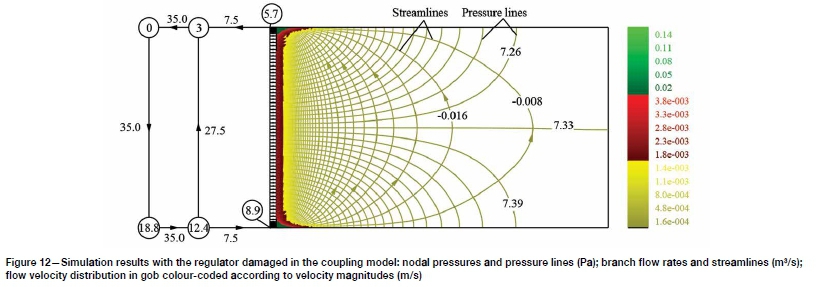
As a scenario analysis, the effects of accidental failure of the regulator in the connection entry between the intake and return entries at the panel recovery end, as shown in Figure 12, is simulated using the developed model. In the simulation, the resistance of the branch with the regulator is 6.1639 Ns²/m⁸, comprising 0.0125 Ns²/m⁸ for the roadway and 6.1514 Ns²/m⁸ for the regulator. The failure of the regulator significantly reduces the branch's resistance to 0.0125 Ns²/m⁸. This simulation shows that the failure of the regulator caused a serious short-circuit of the longwall ventilation system. In comparison to the simulated case before the regulator failure (Figure 8), with 27.5 m³/s of the flow short-circuited to the connection entry, the air flow entering the longwall face after this event is reduced from 30 to 7.5 m³/s -insufficient to ventilate the longwall face. Of the air flowing to the longwall face, the air leaked into the longwall gob is reduced from 138.2 to 18.0 m³/min. If the methane emission in the gob area remains constant, the methane concentration in the air returning to the longwall face at the tailgate T-junction will be about 7.7 times higher than before the failure of the regulator, and is likely to result in more dangerous conditions.

The developed coupling model can be easily modified to facilitate the simulation of the air flow distribution in the bleeder system used in longwall coal mines in the USA. In such a system, a desirable ventilation system is one that keeps the front of explosive methane zone in the gob a sufficient distance away from the longwall face while not over-ventilating the gob in order to avoid conditions for spontaneous combustion. The coupling model can be used to generate appropriate ventilation plans for longwall mining operations.

 

Conclusions

A good understanding of the air flow in the longwall gob behind its operating face is important for mine safety management. An appropriate ventilation system will prevent the methane explosive zone from penetrating into the working face and minimize the zone in which the conditions are favourable for spontaneous combustion. A coupling mine ventilation simulation model that takes into account the interactive relationship between the mine ventilation network (MVN) and gob flow field (GFF) has been developed for studying the air flow patterns in the longwall gob.

(1) A mathematical model that simultaneously couples the 1D MVN and finite element method for 2D/3D GFF for a longwall mine ventilation simulation has been proposed. A computation procedure for solving the resulting equations iteratively has also been proposed.

(2) A program, i-MVS, has been developed based on the proposed mathematical model to implement the required computations. The i-MVS program provides the following two important advantages over the current GFF simulation practices: the GFF is simulated with the ventilation network simultaneously, and no separate and tedious input for the gob boundary conditions is required.

(3) An application simulation was conducted using the developed program. It produces converging and realistic results for the air flows in the longwall face and in the flow field in the longwall gob. The program can be used to generate mining operation and ventilation plans to prevent spontaneous combustion events and avoid explosive methane conditions in the longwall face area.

 

Acknowledgements

This work was supported by Fundamental Research Funds of Shaanxi Province, China [grant numbers 2017JM5039] and the National Natural Science Foundation of China [grant numbers 51574193, 51974232].

 

References

Bear, J. 1972. Dynamics of Fluids in Porous Media. Elsevier, New York.         [ Links ]

Brunner, DJ. 1985. Ventilation models for longwall gob leakage simulation. Proceedings of the 2nd US Mine Ventilation Symposium, Reno, NV. CRC, Boca Raton, FL. pp. 655-662.         [ Links ]

Hartman, H.L., Mutmansky, J.M., Ramani R.V., and Wang, Y.J. 1997. Mine Ventilation and Air Conditioning. Wiley, New York.         [ Links ]

Heinrich, J.C., Huyakorn, P.S., Zienkiewicz, O.C., and Mitchell, A.R. 1977. An 'upwind' finite element scheme for two-dimensional convective transport equation. International Journalfor Numerical Methods in Engineering. vol.11, no.1. pp.131-143.         [ Links ]

Karacan, C.Ö. 2009. Forecasting gob gas venthole production performances using intelligent computing methods for optimum methane control in longwall coal mines. International Journal of Coal Geology, vol. 79. pp. 131-144.         [ Links ]

Li, Z.X., Liu, Y.Z., and Wu, Q. 2008. Improved iterative algorithm for nonlinear seepage in flow field of caving goaf. Journal of Chongqing University, vol. 31. pp.186-190.         [ Links ]

Ozdogan, M.V., Turan, G., Karakus, D., Onur, A.H., Konak,G., and Yalcin, E. 2018. Prevention of spontaneous combustion in coal drifts using a lining material: A case study of the Tuncbilek Omerler underground mine, Turkey. Journal of the Southern African Institute ofMining and Metallurgy, vol. 118. pp. 149-156.         [ Links ]

Shao, Η., Jiang, S.G., and Wang, L.Y. 2011. Bulking factor of the strata overlying the gob and a three-dimensional numerical simulation of the air leakage flow field. Mining Science and Technology, vol. 21. pp. 261-266.         [ Links ]

Saghafi, Α., Bainbridge, N.B., and Carras, J.N. 1995. Modeling of spontaneous heating in a longwall goaf. Proceedings of the 7th US Mine Ventilation Symposium, Littleton, CO. Society for Mining, Metallurgy & Exploration, Littleton, CO. pp. 167-172.         [ Links ]

Saghafi, Α. and Carras, J.N. 1997. Modeling of spontaneous combustion in underground coal mines: application to a gassy longwall panel. Proceedings of the 27th International Conference of Safety in Mines Research Institute, Dhanbad, India. Oxford & IBH Publishing Company, New Delhi. pp. 573-579.         [ Links ]

Schenk, O. and Gartner, K. 2004. Solving unsymmetric sparse systems of linear equations with PARDISO. Journal of Future Generation Computer Systems, vol. 20. pp. 475-487.         [ Links ]

Tripathi, D.D. 2008. New approaches for increasing the incubation period of spontaneous combustion of coal in an underground mine panel. Fire Technology, vol. 44. pp. 185-198.         [ Links ]

Wang, H.G. 2009. Study on superposition method of air leakage and gas delivery in cave-in gobs. PhD dissertation, Xi'an University of Science and Technology.         [ Links ]

Wedding, W.C. 2014. Multi-scale modeling of the mine ventilation system and flow through the gob. PhD. dissertation, University of Kentucky.         [ Links ]

Wu, F.L., Gao, J.N., Chang, X.T., and Li, L.Q. 2016. Symmetry property of Jacobian matrix of mine ventilation network and its parallel calculation model. Journal of China Coal Society, vol. 41. pp. 1454-1459.         [ Links ]

Xia, T.Q., Zhou, F.B., Wang, X.X., Zhang, Y., Li, Y., Kang, J., and Liu, J. 2016. Controlling factors of symbiotic disaster between coal gas and spontaneous combustion in longwall mining gobs. Fuel, vol. 182. pp. 886-896.         [ Links ]

Xia, T.Q., Xu, M.J., and Wang, Y.L. 2017. Simulation investigation on flow behavior of gob gas by applying a newly developed FE software. Environmental Earth Sciences, vol. 76. pp. 485.         [ Links ]

Yang, L., Zheng, J.L., and Zhang, R. 2014. Implementation of road horizontal alignment as a whole for CAD. Journal of Central South University, vol. 21. pp. 3411-3418.         [ Links ]

Yang, Y,L,, Li, Z,H,, and Hou, S.S. 2014. The shortest period of coal spontaneous combustion on the basis of oxidative heat release intensity. International Journal ofMining Science and Technology, vol. 24. pp. 99-103.         [ Links ]

Yuan, L.M. and Smith, A.C. 2008. Numerical study on effects of coal properties on spontaneous heating in longwall gob areas. Fuel, vol. 87. pp. 3409-3419.         [ Links ]

Zhang, C., Tu, S.H., Zhang, L, Bai, Q., Yuan, Y., and Wang, F. 2016. A methodology for determining the evolution law of gob permeability and its distributions in longwall coal mines. Journal of Geophysics and Engineering, vol. 13. pp. 181-193.         [ Links ]

Zhao, Y.S. 1994. Finite Element Method and its Application in Mining Engineering. Coal Industry Press, Beijing        [ Links ]

Zhou, L.H. and Smith, A.C. 2011. Improvement of a mine fire simulation program-incorporation of smoke rollback into MFIRE 3.0. Journal of Fire Sciences, vol. 30. pp. 29-39.         [ Links ]

Zhou, L.H., Smith, A.c., and Yuan, L.M. 2016. New improvements to MFIRE to enhance fire-modeling capabilities. Mining Engineering, vol. 68. pp. 45-50.         [ Links ]

Zienkiewicz, O.C., Taylor, R.L., and Zhu, J.Z. 2015. The Finite Element Method: Its Basis & Fundamentals. 7th edn. World Publishing Corporation, Beijing. pp. 1-5.         [ Links ]

Zienkiewicz, O.C., Taylor, R.L., and Nithiarasu, P. 2014. The Finite Element Method for Fluid Dynamics. 7th edn. Butterworth-Heinemann, Waltham, MA. pp. 31-80.         [ Links ] ♦

 

 

Correspondence:
F-l Wu
15038537@qq.com

Received: 24 Apr. 2018
Revised: 17 Mar. 2019
Accepted: 24 Apr. 2019
Published: October 2019