GEOMETALLURGICAL EDITION

 

Prediction of copper recovery from geometallurgical data using D-vine copulas

 

 

E. Addo Jr^I; A.V. Metcalfe^II; E.K. Chanda^I; E. Sepulveda^{I, V}; W. Assibey-Bonsu^III; A. Adeli^IV

^ISchool of Civil, Environmental and Mining Engineering, University of Adelaide, Australia
^IISchool of Mathematical Sciences, University of Adelaide, Australia
^IIIGroup Geostatiscian and Evaluator, Gold Fields Limited, South Africa
^IVDepartment of Mining Engineering, University of Chile, Chile
^VSchool of Mining Engineering, University of Talca, Chile

Correspondence

 

This paper was first presentedat the Furnace Tapping 2018 Conference, 15–16 October 2018, Nombolo Mdhluli Conference Centre, Kruger National Park, South Africa.

---

SYNOPSIS

The accurate modelling of geometalhirgical data can significantly improve decision-making and help optimize mining operations. This case study compares models for predicting copper recovery from three indirect test measurements that are typically available, to avoid the cost of direct measurement of recovery. Geometallurgical data from 930 drill core samples, with an average length of 19 m, from an orebody in South America have been analysed. The data includes copper recovery and the results of three other tests: Bond mill index test; resistance to abrasion and breakage index; and semi-autogenous grinding power index test. A genetic algorithm is used to impute missing data at some locations so as to make use of all 930 samples. The distribution of the variables is modelled with D-vine copula and predictions of copper recovery are compared with those from regressions fitted by ordinary least squares and generalized least squares. The D-vine copula model had the least mean absolute error.

Keywords: copula, geometallurgy, modelling, regression, mining.

---

 

 

Introduction

In this paper we compare the use of D-vine copula, generalized least squares (GLS), and ordinary least squares (OLS) for modelling geometallurgical data from an orebody in South America. The first objective is to construct models for predicting copper recovery (Rec) from the Bond mill index test (BWi); resistance to abrasion and breakage index (A*b); and semi-autogenous grinding (SAG) power index test (Spi). This involves fitting a D-vine copula and regression models fitted by OLS and GLS. The second objective is to investigate the performance of the fitted models for predicting Rec (Willmott and Matsuura 2005).

Traditional resource model approaches either ignore the mineral processing characteristics of extracted tonnages or treat processing as an independent component of a mining operation. The net present value (or any other objective) can be truly optimized only by considering the mining operation as an integrated system in which net value is defined as the end-product that the company sells. This approach requires the resource model to be extended to include all relevant rock properties and processing responses.

Comminution performances and mineral processing recovery factors have a substantial effect on production and the final value of the product. Hence their prediction in the early stages of a mining operation is crucial. The accurate and precise prediction of these variables is important for mine planning and project risk assessment. Commonly used tests for determining comminution performances are BWi, Spi, and A*b. Better understanding of the physical and chemical principles on which these performance indices are based has contributed to the acceptance and use of geometallurgy in resource modelling, referred to in a wider context as grade engineering.

Lishchuk et al. (2015) define geometallurgy as a multidisciplinary approach that integrates geology, mineralogy, mineral processing, and metallurgy to create spatially based models for production and operational decisions. The primary geological rock properties (e.g., grade, alteration, texture, and grain size) are proxies for predicting metallurgical responses (e..g., type of processing, throughput, recovery, energy consumption, reagent usage, and grindability) (Coward et al. 2009; Dowd, Xu, and Coward, 2016). Incorporating these variables into the resource model in a way that can be used effectively in mine planning poses a challenge to geostatisticians and resource modellers. In most projects, the lack of appropriate geometallurgical data collection and analysis leads to unreliable metallurgical response models.

The relatively large difference between the number of samples recorded in the geological database (logging, assays etc.) and the relatively few metallurgical test work samples further hinders the integration of metallurgical responses into the resource model using existing geostatistical methods (Hunt, Kojovic, and Berry, 2013). Also, there is often the problem of missing values of metallurgical variables, which may not be measured at all locations. Retaining only data where all variables are sampled could result in removing a large amount of data from the geometallurgical programme (Deutsch, 2013), which can lead to poor geostatistical modelling in areas where more data (of some variables) is actually sampled.

In addition, most geological and geometallurgical variables have complex multivariate relationships that are the result of a succession of several chaotic, nonlinear natural processes which are often not well modelled by parametric multivariate probability distribution (Deutsch 2013). Moreover the nonadditive and compositional nature of geological/geometallurgical variables makes their modelling more difficult (Walters and Kojovic 2006; Williams and Richardson, 2004). An alternative modelling strategy that can capture all these complex multivariate relationships is crucial for successful modelling of geometallurgical variables. Multivariate D-vine copulas are ideal for modelling complex multivariate relationships, skewed distributions, and tail-dependent distributions. Moreover, the D-vine copula models encompass all multivariate distribution, including the multivariate Gaussian distribution (MVG).

This paper is comprised of three main sections. The 'Method' section describes the theory of copulas, pair copulas, and vine copulas (D-vine) construction models. The 'Application' section describes data imputation, modelling of copper recovery in terms of A*b, BWi, and Spi, and finally the prediction of copper recovery from A*b, BWi and Spi. This is followed by the 'Discussion and Conclusion'.

 

Method

This section gives an overview and summarizes the principles of copulas, pair copulas (D-vine) construction for four variables. Further details about the concept of copulas can be found in Joe (1996) and Nelsen (2006). In addition, more detailed explanation of the pair copula and vine copula models can be found in Aas et al. (2009), Bedford and Cooke (2002), and Kurowicka and Cooke (2006). Spatial applications of pair copulas can be found in Gräler and Pebesma (2011), Gräler (2014), Musafer et al. (2013), Musafer and Thompson (2016), and Addo, Chanda, and Metcalfe (2018).

Theory of copulas

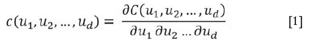
A copula is a multivariate uniform distribution. It follows that any multivariate distribution has a copula form because the marginal cumulative distribution functions (cdfs) can be transformed to uniform distributions. Conversely, the uniform margins of any copula can be transformed to any continuous probability distributions, which can differ for different margins. Therefore copulas provide a very flexible approach in modelling multivariate data. Consider a random variable Z= {z_x,...,z) and define u=F(z). We can define a copula by its cdf C(u,,u₂,...,u) and the corresponding probability density function (pdf) is

The copula pdf links the marginal pdfs to the multivariate pdf:

Generally, we often require multivariate distributions of more than two variables. The elliptical copulas (i.e. Gaussian and Student-t copula) can easily be extended to more than two variables, but this is not generally the case for the Archimedean copulas ( i.e. Clayton, Frank, and Gumbel copula). A more flexible approach to modelling such multivariate distributions is the pair-copula D-vines as described by Aas et al. (2009), Bedford and Cooke (2002), and Kurowicka and Cooke (2006).

Pair copula

Any multivariate distribution can be factorized in different ways using its conditional distributions. Specifically, a copula can be factorized as a product of the marginal distributions and the bivariate conditional copulas. We often term such factorization 'pair-copula models'. Joe (1996) presented a construction for a pair-copula model for a multivariate copula based on the distribution functions. After Joe's construction of a copula based on the distribution functions, Bedford and Cooke (2002) also presented a construction in terms of the densities. In their work, they organized the constructions in a graphical way involving a sequence of nested trees, which they refer to as 'regular vines'. They defined two popular classes of pair-copula construction (PCC) models, which they refer to as the D-vines and canonical (C) vines. Their work was further developed by Kurowicka and Cooke (2006). The derivation of a D-vine model, which is used in this application, is outlined below.

D-vines

Generally the pair copula can be seen as a multivariate copula that aims to approximate the target copula, since not all copulas can be expressed as a vine copula (Haff, Aas, and Frigessi, 2010). This decomposition is, however, not unique; for example, a five-dimensional density can have about 240 different constructions. In the D-vines, the decomposition of the joint density consists of the pair-copula densities evaluated at conditional distributions functions and for specified indices and marginal densities (Bedford and Cooke 2002; Czado 2010 and Gräler 2014). Figure 1, which is reproduced from Aas et al. (2009), shows the graphical model used to demonstrate the D-vines for four variables. This consists of three trees: T_j. j=1,2,3.

 

 

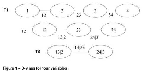
Tree T_j. has n+1-j nodes, where n is the number of variables.

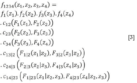
Using the decomposition shown in Figure 1 and Equation [3], the joint density function of four random variables can be expressed using the D-vines asw

As shown in Equation [3], the D-vine distribution requires the computation of several conditional distribution functions and conditional bivariate copulas. From Joe (1996) and Aas, Frigessi, and Bakken (2009), the conditional distribution functions F(z\v).

for an m-dimensional vector v=(v₁...,v_m) can be obtained from the following recursive relationship:

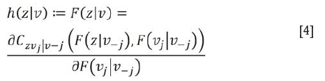
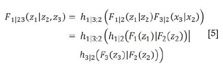
where Vj [j=1,...,m) is an arbitrary component of v, and v(-j)= (v₁,...,vj-1),vj+1),...,v_m) denotes the vector v excluding element Vj. The bivariate copula function is also specified by C(zVj I vj). Given u_i(/=1,...,n) to denote F_t (z_t), we can derive the conditional distribution function F(u₃ I u₁,u₂) that is needed as an argument for C_14I23 in a four-dimensional D-vine copula density using Equation [4]. From Figure 1 Tree 3 (73) the argument C_14I23, namely F_1I23(x₁I x₂,x₃), can be evaluated using the h function (Kraus and Czado 2016) associated with C₁₃₂,C₁₂,and C₂₃ from the first two trees T₁ and T₂ as

D-vine copula-based conditional forecasting model

With the defined conditional distributions function in Equation [5], the inverse forms can also be defined, and can be used in forecasting. Using the bivariate case, the conditional distribution function of two random variables z₁ and z₂ is h (u₂Iu₁). The main goal is to be able to obtain u₂based on the information available at u₁. Given some fixed probabilities τ, we can derive u₂ from

C(u₂Iu₁)using an explicit function u₂ = u₂ = C u2_Iu1(t;u₁)= h¹(tlu₁), where C _u¹_2Iu1is the inverse of the copula function known as the quantile curve of the copula (Xu and Childs, 2013). The xth copula-based conditional quantile function of variable z₂is

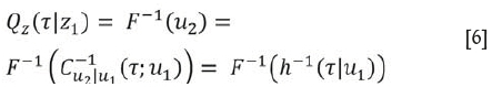
where F -¹is the inverse of u₂. For the four-dimensional case, the xth conditional quantile function of z₄, Q_x4 (x\z_l,z₂,z₃) can be deduced by the recursive computation

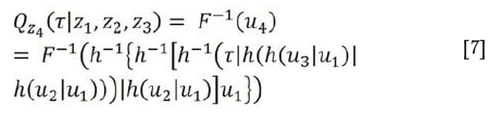
Hence we can forecast z₄ based on the variables z₁,z₂, and z₃. Moreover, Q_z4(x\z_l,z₂,z₃) is monotonically increasing in τ so the crossing of quantile functions corresponding to different quantile levels is not possible. Bernard and Czado (2015) proved that linear regression quantile functions may cross if a non-Gaussian data is modelled.

In general, the multivariate D-vine copula model for the four-dimensional vine model can be implemented by following the steps below. Further details of the method can be found in Kraus and Czado (2016) and Liu et al. (2015).

1. Fit an appropriate marginal distribution to each of the variables, z₁,z₂,z₃, and z₄, where z₄is the predicted variable and all the others are the explanatory variables.

2. Model the joint dependence structure of all the four variables using Equation [5] for the D-vine model.

3. Estimate all the appropriate bivariate copula for each pair copula using the R library VineCopula ( Schepsmeier et al., 2015).

4. Estimate the conditional distribution function of variable z₄ conditioned on the given variables z₁,z₂,z₃using Equation [5].

5. Finally, generate the predicted values of z₄based on the given variable, z₁,z₂,z₃using the copula-based quantile function as given in Equation [7].

Performance of models

The mean absolute error (MAE) and root mean square error (RMSE) have been used to assess the prediction performance of the models.

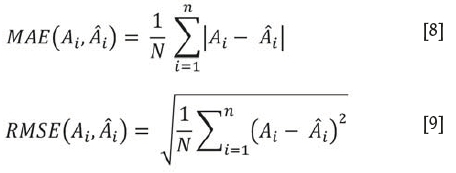
where A_tis the observed recovery, and A_tis the predicted recovery obtained using a fitted model to all N =930. So, the performance measures are calculated within the entire sample.

 

Application

Nine hundred and thirty (with some missing values) drill core samples with an average length of 19 m from a mine in South America were sampled for geometallurgical attributes of copper recovery (Rec), Bond mill index test (BWi), resistance to abrasion and breakage index (A*b), and semi-autogenous grinding power index test (Spi). Typical of most geometallurgical data-sets, there are missing values that have not been sampled at some locations. There are 299 non-missing data-sets that are sampled at all locations. To be able to use all 930 georeferenced drill core samples for the analysis, we employed a data imputation algorithm to predict missing values at some locations.

Data imputation

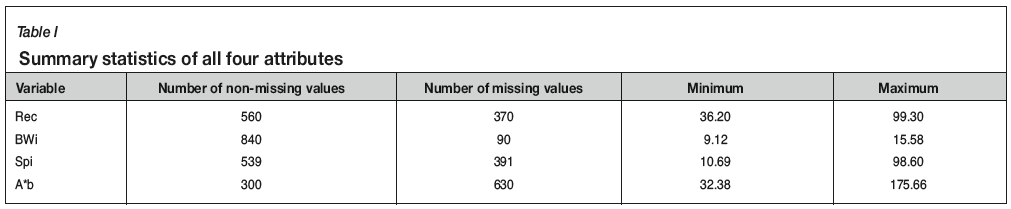
The data-set has 930 georeferenced samples with four attributes of interest: Rec, BWi, Spi, and A*b. Table I shows the summary of descriptive statistics for all four attributes.

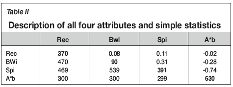
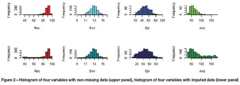
Data imputation was formulated as an optimization problem seeking to preserve two main properties: the reproduction of the individual histograms and the bivariate correlation among the variables. Histograms of each of the variables were calculated using non-missing (informed) values, and correlations were calculated using samples where all variables have non-missing values. Table II indicates the bivariate correlations, and number of missing and non-missing values for the pair attributes. The diagonal shows the number of missing values, the upper triangle shows the Pearson correlation between two attributes, and the lower triangle shows the number of non-missing values for the pair attributes.

 

 

The data-sets were decomposed in two sets: non-missing (informed) values and missing values. Hence, the multivariate data-set was defined as: X= {X_V...,X_D}, where D is the number of attributes. Each X is also defined as follows: X = V _iυ M_t, where V and M_irepresent the informed and missing values respectively, and V_tυ M_iis used to indicate V _iif available, or M_iotherwise.

The histogram function used for the imputation was denoted by H(X), and used 21 regular bins or class intervals. The correlation is given by

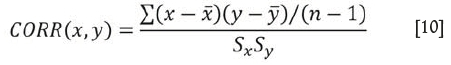
where x,y,S, and S are the mean and standard deviation of x and y, and n is the sample size.

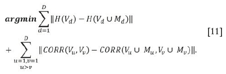
The optimization problem for the data imputation was formulated as follows.

Decision variables

As the main objective is to impute values to all missing values, the decision variables correspond to the set {M_V...,M_D}. According to Table I, there are 1481 missing values to impute.

Objective function

Minimization of the mean quadratic error between the histogram of each variable with and without imputed data and the mean quadratic error between the correlations of each pair of variables with and without the imputed data.

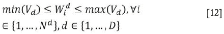
Constraints

The only imposed constraint is the lower and upper bounds for each attribute, for which the minimum and maximum values are observed from the samples.

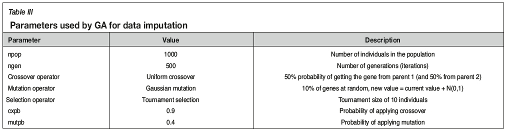
This formulation is nonlinear and may have no unique solution. Metaheuristics are optimization methods that can deal with these kinds of problems successfully. We therefore solved the optimization formulation by genetic algorithm (GA) metaheuristics due to its flexibility and good performance (Whitley, 1994). The GA is a stochastic method, hence different seeds of random number generator may generate different solutions. In this application, our experiments show that the imputed values change slightly in response to varying the seed, but the histograms and correlations are very stable. We use one representative set of imputed data found by one execution of GA. Table III shows the parameters used in the GA for data imputation.

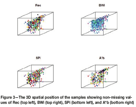
The Pearson's correlation computed for imputed and non-missing samples shows that the correlations were perfectly reproduced. Figure 2 (upper and lower panel) shows the histogram of the imputed data and with non-missing values respectively. Figure 3 also shows all four non-missing variables (i.e., Rec, BWi, Spi, and A*b) in space. We discuss Figure 3 under the 'Discussion and Conclusion' section.

 

 

Analysis

The imputed data, consisting of 930 drill core samples for four variables (Rec, BWi, Spi, and A*b), was used for the analysis, the explanatory variables being Spi, BWi, and A*b. The hypothesis of stationarity was tested by fitting a regression of recovery on the mean corrected eastings (x), mean corrected northings (y), mean corrected elevations (z), x², y², and the cross-product xy in Equation [13]. This model, referred to as Modell, is

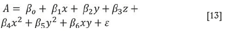
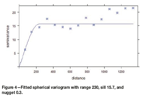
where ε is the random error, which is expected to be spatially correlated, with mean of zero and standard deviation a_o. Modell was initially fitted by OLS. Then, a spherical variogram was fitted to the residuals and the variogram parameters were used for fitting with a GLS functiongls( ) in the R library nlme (Pinheiro and DebRoy, 2016). The fitted spherical variogram and model parameters are shown in Figure 4. The estimated coefficients for the GLS fit to Model1 are shown in Table IV.

 

 

 

 

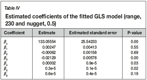
The standard deviation of the residuals is 14.26 on 923 degrees of freedom, which is smaller than the standard deviation of the recovery data (15.02). While this reduction in standard deviation is small, the sample size is relatively large and two of the coefficients in the fitted quadratic surface are highly significant statistically. We then assume the residuals from the GLS regression are a realization of a stationary spatial process.

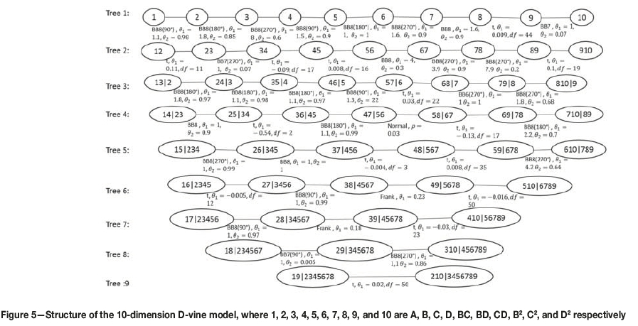
The residuals from the model res (Rec) were taken as the response variable for recovery (Rec) and were used together with the BWi, Spi, and A*b (referred to as B,C, and D respectively) to fit the D-vine copula. Variables B,C, and D were mean-corrected to avoid the excessively large values of quadratic terms and ill-conditioned matrices that would result if the original data was used. Quadratic terms and interactions between the explanatory variables included were BD, CD, B², C², D². So a 10-dimensional D-vine based model was constructed, which is made up ofres(Rec), B, C, D, BC, BD, CD, B², C²,and D². In the following, the res(Rec) will be referred to as A.

We fitted an appropriate kernel marginal distribution to each of the mean-corrected variables. After obtaining well-fitted marginal distributions, a 10-dimensional D-vine copula was used to join the margins and model the joint dependence structure. To be able to establish the 10-dimensional D-vine copula, we fitted the best fitting bivariate copula for each pair copula using the R library CDVine developed by Schepsmeier and Brechman (2015). The fitting was done by equating the Kendall's tau to the value of Kendall's tau implied by the dependence parameter (θ₁, θ₂, and ρ), which is referred to as the 'method of moments'. A limitation of the method of moments is that it does not lead easily to a criterion for choosing between the copula forms. Therefore, the method of maximum likelihood was used for choosing between the copula forms, the form with the highest likelihood being chosen. The rotated version of the bivariate copulas (i.e., BB6, BB7, and BB8) with angles 90°, 180°, and 270° was selected by maximum likelihood. In addition, Student-t, normal, and Frank copulas were also selected using maximum likelihood for some trees. Figure 5 illustrates the fitted bivariate copulas and their fitted dependence parameters (θ₁, θ₂, ρ, and df) for the 10-dimensional D-vine model. The final forecasting performance of the 10-dimensional D-vine copula model was calculated using a 10D version of Equation [7]. The predicted values were back-transformed to the original unit (recovery per cent, Rec) by adding the predicted values from the 10D model to the predicted values from Model1.

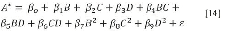
We compared the predicted recovery from the 10-dimensional D-vine copula with an OLS regression and a GLS regression model. The residual from model, referred to in this application as A, which is the response variable, was regressed on the explanatory variables B, C, D, BC, BD, CD, B², C²,and D². Equation [14] shows the OLS regression model fitted, and Table V shows the estimated coefficients for the OLS regression.

 

 

 

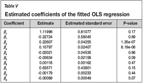
The linear regression model was used to predict recovery and the predicted values were back-transformed to the original units (recovery per cent, Rec) by adding the predicted values from Model1.

The residual from the model referred asA was regressed on the explanatory variables B, C, D, BC, BD, CD, B²,C²,and D² using the GLS model with spherical variogram parameters of range: 230, nugget: 0.5, and sill: 15.7. The GLS model is given in Equation [14], and the estimated model coefficients are shown in Table VI.

 

 

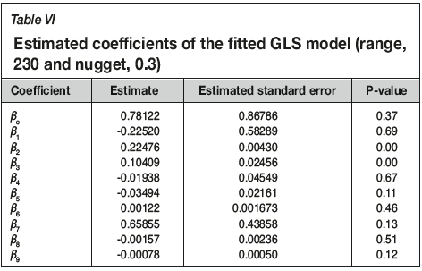
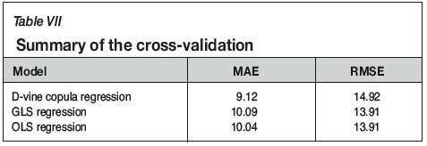
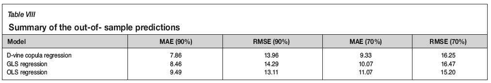
The GLS model was used to make predictions of recovery at each point, and the predicted value was back-transformed to the original unit (recovery per cent Red) by adding the predicted values from Model1. A summary of the cross-validation results using all three models is presented in Table VII. There is little difference between the GLS and OLS fits. The D-vine performs better according to the MAE but not according to RMSE. We discuss this in the next section. Figure 6 illustrates a scatter plot of the observed versus predicted recoveries from the GLS, D-vine, and OLS models. Further comparisons were made by making out-of-sample predictions. Proportions of 10% and 30% were removed at random locations from the 930 complete geometallurgical data. The models (OLS, GLS and D-vine) were fitted to the remaining 90% and 70% of the data.

 

 

Out-of-sample predictions were generated and compared with the known values of the data removed. Figure 7 shows box plots of the removed CuRec (A) and the out-of-sample predictions using OLS (B), GLS (C) and D-vine (D), for 90% and 70% data used for predictions. Summary statistics are given in Table VIII.

 

 

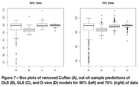
The D-vine performs best in terms of MAE, and GLS regression is an improvement on OLS regression, in terms of MAE for both 10% and 30% data removed. However, OLS regression is slightly better than both the D-vine copula and GLS regressions in terms of RMSE.

 

Discussion and conclusion

Data on four variables (Rec, BWi, Spi, and A*b) from 930 drill core samples at know locations was available. Two hundred and ninety-nine drill cores had a complete record, but there were some missing items from the other 631 cores. In order to use all 930 drill core samples, a genetic algorithm (GA) was used to impute missing items at these locations. The objective function formulated in this case study was designed to reproduce precisely the individual histograms and the linear correlations between pairs of variables. This criterion is, however, subjective and in cases when missing data comes from preferential sampling, the histogram of the imputed data may differ from the actual underlying distribution. For example, it is common to perform metallurgical test work only in ore zones with a high grade profile, hence recovery for low-grade zones will not be well represented in the distribution. The objective function in the data imputation method should be adjusted according to the knowledge of the data-sets. The recovery (Rec), the response in this application, shows a slight, but statistically significant, nonstationarity. The nonstationarity of Rec has been accounted for by fitting a quadratic trend regression surface by the GLS model, with a spherical variogram to approximate the spatial correlation. The residuals from the GLS model were considered as a realization of a stationary process.

The residuals from the model and the mean corrected values for BWi, Spi, and A*b, together with two variable interactions and squares for the three variables, were used to fit a 10-dimensional D-vine copula model. The fitted 10-dimensional D-vine copula model was used to predict recovery, and MAE and RMSE were calculated. These predictions were compared with predictions from regressions fitted by OLS and GLS. The D-vine copula model had the smallest MAE. However, the regression models had lower RMSE. A comparison of the scatter plots suggests that the D-vine gives more accurate and precise predictions for high levels of copper recovery. However, the D-vine appears to overestimate the copper recovery at low levels rather more than the regression models. Out-of-sample predictions using the three models were compared as a further check on the D-vine copula regression model. A proportion of the data (i.e. 10% and 30%) was removed at random locations from the complete geometallurgical datasets. The models were fitted to the remaining 90% and 70% of the data, and out-of-sample predictions were estimated and compared with the known values of 10% and 30% data removed. Results from the analysis shows that the D-vine model had the least MAE for both 90% and 70% data, although OLS regression was slightly better on RMSE. An explanation for the finding that the D-vine copula is better on MAE yet slightly worse on RMSE is that the D-vine copula is less affected by outliers. The outliers will make a major contribution to the RMSE, and regression fits the coefficients by minimizing the RMSE. This has the effect that outlying observations are highly influential in the fitting process, drawing the fitted surface towards them and so reducing the RMSE. For this reason the MAE is considered more useful in the mining industry, where outlying values are common and the implicit assumption of a Gaussian distribution, under which GLS would be optimum, is not realistic. The D-vine copula is preferable to capping, which introduces a downward bias. Moreover, the D-vine will generally produce more accurate prediction intervals than a regression model, because it allows for a general form of the distribution of the errors. Generally, geometallurgical tests are expensive and a modelling approach that can provide accurate and precise predictions of some variables from others will save money.

 

Acknowledgements

This research is supported by an Australian Government Research Training Program Scholarship awarded to Emmanuel Addo Jr. The authors thank the mining company for providing the geometallurgical data-sets used in this case study. We express our gratitude to the reviewers for their comments and suggestions, which have improved the practical application of this manuscript.

 

References

Aas, K., Czado, C., Frigessi, A., and Bakken, H. 2009. Pair-copula constructions of multiple dependence. Insurance: Mathematics and Economics, vol. 44, no. 2. pp. 182-198.         [ Links ]

Addo, E., Chanda, E., and Metcalfe,A.V. Spatial pair-copula model of grade for an anisotropic gold deposit. Mathematical Geosciences, July. pp. 1-26. doi: 10.1007/s11004-018-9757-7        [ Links ]

Bedford, T. and Cooke, R.M. 2002. Vines: A new graphical model for dependent random variables. Annals of Statistics, vol. 30, no. 4. pp. 1031-1068.         [ Links ]

Bernard, C. and Czado, C. 2015. Conditional quantiles and tail dependence. Journal of Multivariate Analysis, vol. 138. pp. 104-126.         [ Links ]

Coward, S., Vann, J., Dunham, S., and Stewart, M. 2009. The Primary-Response framework for geometallurgical variables. Proceedings of the 7th international Mining Geology Conference, Perth, WA, 17-19 August 2009. Australasian Institute of Mining and Metallurgy, Melbourne. pp. 109-113.         [ Links ]

Deutsch, C.V. 2013. Geostatistical modelling of geometallurgical variables - problems and solutions. Proceedings of the Second AusIMM International Geometallurgy Conference, Brisbane, QLD, 30 September - 2 October 2013. Australasian Institute of Mining and Metallurgy, Melbourne. pp. 7-16.         [ Links ]

Dowd, P., Xu, C., and Coward, S. 2016. Strategic mine planning and design: some challenges and strategies for addressing them. Mining Technology, vol. 125, no. 1. pp. 22-34.         [ Links ]

Erhardt, T.M., Czado, C., and Schepsmeier, U. 201). R-vine models for spatial time series with an application to daily mean temperature. Biometrics, vol. 71, no. 2. pp. 323-332.         [ Links ]

Fenske, N., Kneib, T., and Hothorn, T. 2011. Identifying risk factors for severe childhood malnutrition by boosting additive quantile regression. Journal of the American Statistical Association, vol. 106, no. 494. pp. 494-510.         [ Links ]

Gräler, Β. 2014. Developing spatio-temporal copulas. PhD dissertation, Institute for Geoinformatics, University of Münster.         [ Links ]

Gräler, Β. and Pebesma, E. 2011. The pair-copula construction for spatial data: a new approach to model spatial dependency. Procedia Environmental Sciences, vol. 7. pp. 206-211.         [ Links ]

Haff, I.H., Aas, K., and Frigessi, A. 2010. On the simplified pair-copula construction-simply useful or too simplistic? Journal of Multivariate Analysis, vol. 101, no. 5. pp. 1296-1310.         [ Links ]

Hunt, J., Kojovic, T., and Berry, R. 2013. Estimating comminution indices from ore mineralogy, chemistry and drill core logging. Proceedings of the Second AusIMM International Geometallurgy Conference, Brisbane, QLD, 30 September - 2 October 2013. Australasian Institute of Mining and Metallurgy, Melbourne. pp. 173-176.         [ Links ]

Joe, H. 1996. Families of m-variate distributions with given margins and m (m-1)/2 bivariate dependence parameters. Lecture Notes - Monograph Series. Institute of Mathematical Statistics, Hayward, CA. pp. 120-141. https://projecteuclid.org/euclid.lnms/1215452614        [ Links ]

Kraus, D. and Czado, C. 2016. D-vine copula based quantile regression. Computational Statistics and Data Analysis. https://arxiv.org/abs/1510.04161v4        [ Links ]

Kurowicka, D. and Cooke, R.M. 2006. Uncertainty Analysis with High Dimensional Dependence Modelling. Wiley.         [ Links ]

Lishchuk, v., Koch, P-H., Lund, C., and Lamberg, P. 2015. The geometallurgical framework. Malmberget and Mikheevskoye case studies. Minerals and Metallurgical Engineering Division, Luleâ University of Technology.         [ Links ]

Liu, Z., Zhou, P., Chen, X., and Guan, Y. 2015. A multivariate conditional model for streamflow prediction and spatial precipitation refinement. Journal of Geophysical Research: Atmospheres, vol. 120, no. 19. https://doi.org/10.1002/2015JD023787        [ Links ]

Musafer, G.N. and Thompson, M.H. 2016. Non-linear optimal multivariate spatial design using spatial vine copulas. Stochastic Environmental Research and Risk Assessment, vol. 31, no. 2. pp. 551-570.         [ Links ]

Musafer, G.N., Thompson, M.H., Kozan, E., and Wolff, R.C. 2013. Copula-based spatial modelling of geometallurgical variables. Proceedings of the Second AusIMM International Geometallurgy Conference, Brisbane, QLD, 30 September - 2 October 2013. Australasian Institute of Mining and Metallurgy, Melbourne. pp 239-246.         [ Links ]

Nelsen, R. 2006. An introduction to copulas. Lecture Notes in Statistics. Springer, New York.         [ Links ]

Pinheiro, J., Bates, D., DebRoy, S., Sarkar, D., and R Core Team. 2016. _nlme: Linear and nonlinear mixed effects models_. R package version 3.1-128. http://CRAN.R-project.org/package=nlme        [ Links ]

Schepsmeier, U., Stöber, J., Brechmann, E.C., Graeler, Β., Nagler, T., and Erhardt, T. 2016. VineCopula: Statistical inference of vine copulas. R package version 2.0.5. https://github.com/tnagler/VineCopula        [ Links ]

Walters, S. and Kojovic, T. 2006. Geometallurgical mapping and mine modelling (GEMIII) - the way of the future. Proceedings of SAG 2006, Vancouver, Canada, 23-27 September 2006. vol. 4. pp. 411-425.         [ Links ]

Whitley, D. 1994. A genetic algorithm tutorial. Statistics and Computing, vol. 4, no. 2. pp. 65-85.         [ Links ]

Williams, S.R. and Richardson, J. 2004. Geometallurgical mapping: A new approach that reduces technical risk. Proceedings of the 36th Annual Meeting of the Canadian Mineral Processors. Canadian Institute of Mining, Metallurgy and Petroleum, Montreal. pp. 241-268.         [ Links ]

Willmott, C.J. and Matsuura, K. 2005. Advantages of the mean absolute error (MAE) over the root mean square error (RMSE) in assessing average model performance. Climate Research, vol. 30, no. 1. pp. 79-82.         [ Links ]

Xu, Q. and Childs, T. 2013. Evaluating forecast performances of the quantile autoregression models in the present global crisis in international equity markets. Applied Financial Economics, vol. 23, no. 2. pp. 105-117.         [ Links ]

 

 

Correspondence:
E. Addo Jr
emmanuel.addojunior@adelaide.edu.au

Received: 10 Sep. 2018
Revised: 1 Apr. 2019
Accepted: 1 Apr. 2019
Published: April 2019