PAPERS OF GENERAL INTEREST

 

Investigation of flow regime transition in a column flotation cell using CFD

 

 

I. Mwandawande^I; G. Akdogan^I; S.M. Bradshaw^I; M. Karimi^II; N. Snyders^I

^IUniversity of Stellenbosch, South Africa
^IIDepartment of Chemistry and Chemical Engineering, Chalmers University of Technology, Sweden

 

 

---

SYNOPSIS

Flotation columns are normally operated at optimal superficial gas velocities to maintain bubbly flow conditions. However, with increasing superficial gas velocity, loss of bubbly flow may occur with adverse effects on column performance. It is therefore important to identify the maximum superficial gas velocity above which loss of bubbly flow occurs. The maximum superficial gas velocity is usually obtained from a gas holdup versus superficial gas velocity plot in which the linear portion of the graph represents bubbly flow while deviation from the linear relationship indicates a change from the bubbly flow to the churn-turbulent regime. However, this method is difficult to use when the transition from bubbly flow to churn-turbulent flow is gradual, as happens in the presence of frothers. We present two alternative methods in which the flow regime in the column is distinguished by means of radial gas holdup profiles and gas holdup versus time graphs obtained from CFD simulations. Bubbly flow was characterized by saddle-shaped profiles with three distinct peaks, or saddle-shaped profiles with two near-wall peaks and a central minimum, or flat profiles with intermediate features between saddle and parabolic gas holdup profiles. The transition regime was gradual and characterized by flat to parabolic gas holdup profiles that become steeper with increasing superficial gas velocity. The churn-turbulent flow was distinguished by steep parabolic radial gas holdup profiles. Gas holdup versus time graphs were also used to define flow regimes with a constant gas holdup indicating bubbly flow, while wide gas holdup variations indicate churn-turbulent flow.

Keywords: flotation column, maximum superficial velocity, flow regime, bubbly flow, transition, churn-turbulent flow.

---

 

 

Introduction

Two types of flow can be distinguished in gas-liquid flows in bubble columns: bubbly flow and churn-turbulent flow. The bubbly flow regime is characterized by uniform flow of bubbles of uniform size. Churn-turbulent flow, on the other hand, is characterized by a wide variation in bubble sizes with large bubbles rising rapidly and causing liquid circulation.

Flotation columns are normally operated in the bubbly flow regime, which is the optimal condition for column flotation (Finch and Dobby, 1990; Yianatos and Finch, 1990; Ityokumbul, 1992). However, it has been generally observed that flotation column performance deteriorates when the superficial gas velocity is increased beyond a certain limit where the flow regime changes from bubbly flow to churn-turbulent flow (Xu, Finch, and Uribe-Salas, 1991). The identification of this critical or maximum superficial gas velocity is therefore important for optimal operation of flotation columns.

Xu, Finch, and Uribe-Salas (1991) and Xu et al. (1989) investigated three phenomena that can be used to identify the maximum superficial gas velocity in column flotation: loss of interface, loss of positive bias flow, and loss of bubbly flow. Loss of interface occurs when the hydrodynamic conditions in the froth zone of the column become identical to the conditions prevailing in the collection zone. This will result in the loss of the cleaning action associated with the froth zone.

In column flotation, wash water, which is continuously added at the top of the column, maintains a net downward flow of water that prevents entrained particles from reaching the concentrate. This net downward flow of water is referred to as positive bias flow. By minimizing entrainment of unwanted particles, a positive bias maximizes the concentrate grade. Loss of positive bias occurs when the superficial gas velocity is high enough to cause a reversal of the net flow of water at the froth/collection zone interface.

On the other hand, the loss of bubbly flow occurs when the superficial gas velocity is sufficiently high to bring about a transition from bubbly flow conditions to churn-turbulent flow. The increased mixing associated with churn-turbulent flow is unfavourable for mineral recovery in the column.

Considering the froth and liquid (pulp) phases as distinct flow regimes with different liquid holdups, Langberg and Jameson (1992) investigated the hydrodynamic conditions under which the froth and pulp phases can coexist in a flotation cell. The effects of superficial gas velocity and bubble size on the limiting conditions for flow regime coexistence and for countercurrent flow across the froth-liquid interface were studied using a one-dimensional two-phase flow model. Their study identified two hydrodynamic limiting conditions relevant to the operation of flotation cells and columns: the limiting condition for the coexistence of the froth and liquid (pulp) phases, and the limiting condition for countercurrent flow.

Of the three phenomena used to identify the maximum superficial gas velocity in column flotation, the loss of bubbly flow is the most difficult to determine (Xu, Finch, and Uribe-Salas, 1991; Xu et al., 1989). The relationship between gas holdup and superficial gas velocity is used to determine the loss of bubbly flow in the column. In this method, a linear gas holdup versus superficial gas velocity relationship represents bubbly flow while deviation from linearity defines loss of bubbly flow. However, the loss of bubbly flow is difficult to identify using this method because of the gradual nature of the transition from bubbly flow to churn-turbulent conditions in the presence of frother (Xu et al., 1989). During the transition from bubbly flow to churn-turbulent flow, the bubble size increases rapidly due to bubble coalescence. However, the presence of frothers suppresses bubble coalescence, causing the transition to churn-turbulent flow to become gradual.

In this research, the maximum superficial gas velocity for transition from bubbly flow to churn-turbulent flow was studied using computational fluid dynamics (CFD). Besides the gas holdup versus superficial gas velocity relationship, two alternative methods of flow regime characterization were employed to identify the loss of bubbly flow in a pilot-scale column flotation cell. The first method involves examining the evolution of radial gas holdup profiles as a function of superficial gas velocity. The shape of the radial gas holdup profile has been recognized as a function of the flow pattern in two-phase flows (Kobayasi, Iida, and Kanegae, 1970; Serizawa, Kataoka, and Michiyoshi, 1975). A graph of gas holdup versus time can also be used to identify the prevailing flow regime in the flotation column (Shen, 1994). Wide variations in the gas holdup versus time graph characterize churn-turbulent flow conditions, while gas holdup is almost constant under bubbly flow conditions.

 

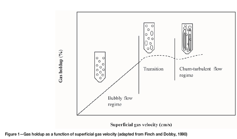
Methods for flow regime identification

The relationship between gas holdup and superficial gas velocity can be used to define the prevailing flow regime in the flotation column (Finch and Dobby, 1990). In the bubbly flow regime, the gas holdup increases linearly with increasing superficial gas velocity. However, the gas holdup deviates from this linear relationship when the superficial gas velocity is increased above a certain value, as shown in Figure 1. The superficial gas velocity at which deviation from the linear relationship occurs is thus the maximum or critical velocity, above which the flow regime changes from bubbly flow to churn-turbulent flow. In other words, it is the maximum superficial gas velocity for loss of bubbly flow.

Xu et al. (1989) applied the gas holdup versus superficial gas velocity relationship to determine the maximum superficial gas velocity for loss of bubbly flow in a pilot-scale flotation column. However, they reported difficulties in the identification of the regime transition point as a result of the gradual nature of this transition, particularly in the presence of frother. The present study therefore applies the following alternative methods to distinguish the different flow regimes and thus identify the maximum velocity above which the transition from bubbly flow to churn-turbulent flow will occur.

Radial gas holdup profiles

Two general gas holdup profiles are known to exist, the parabolic profile and the saddle-shaped profile. Kobayasi, Iida, and Kanegae (1970) studied the characteristics of the local void fraction (gas holdup) distribution in air-water two-phase flow. They reported a 'peculiar' distribution, different from the previously accepted power law distribution in bubbly flow conditions. The distribution associated with bubbly flow had its peaks near the pipe wall. On the other hand, the distribution in slug flow had its maximum at the centre of the pipe.

Serizawa, Kataoka, and Michiyoshi, (1975) also studied various local parameters and turbulence characteristics of concurrent air-water two-phase bubbly flow. They found that the distribution of void fraction (radial gas holdup) was a strong function of the flow pattern. The void fraction distribution changed from saddle-shaped to parabolic as the gas velocity increased. A saddle-shaped distribution is therefore associated with bubbly flow conditions, while a parabolic one represents slug flow.

Gas holdup versus time graph

A plot of gas holdup versus time can also be used to identify the existing flow regime in a column The gas holdup versus time will be relatively constant when the column is in the bubbly flow regime. On the other hand, the gas holdup will show wide variations when the column is operating in the churn-turbulent regime (Shen, 1994). A similar method has been used by previous researchers who used variations in conductivity signals to characterize the flow regime in the downcomer of a Jameson flotation cell (Mecklenburg, 1992; Summers, 1995).

 

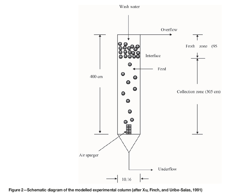
Description of the column

The CFD model developed in the present research was used to simulate the flotation column that was used in the experimental work of Xu, Finch, and Uribe-Salas (1991) and Xu et al. (1989). The column was made of Plexiglas and was 400 cm in height and 10.16 cm in diameter. The column was operated continuously, with air introduced into the bottom of the column through a cylindrical stainless steel sparger, 3.8 cm in diameter and 7 cm in length. This sparger geometry gives a ratio of column cross-section to sparger surface area of about 1:1. A schematic diagram of the column is presented in Figure 2. A detailed description of the experimental set-up is presented in Xu, Finch, and Uribe-Salas (1991).

 

CFD methodology

Multiphase model

A Eulerian-Eulerian (E-E) multiphase modelling approach was used in this study. The Eulerian-Eulerian model was selected on the basis of its lower computational cost compared to other modelling approaches such as the volume of fluid (VOF) and the Eulerian-Lagrangian methods. A VOF model would entail tracking of the interface between different phases, while the Eulerian-Lagrangian method would involve tracking of the motion of individual bubbles using an equation of motion. Both of these methods are therefore not suitable for systems that involve large numbers of bubbles, such as those in the present research. In the E-E approach, both the continuous phase and the dispersed phase are considered as interpenetrating continua and both are modelled in the Eulerian frame of reference. The equations for conservation of mass and momentum are then solved for each phase separately. In this study, the two-phase flow was modelled considering water as the continuous phase (or primary phase) and air bubbles as the dispersed phase (or secondary phase).

Interaction between the phases was accounted for by inclusion of the drag force between phases. The drag force is included in the respective conservation of momentum equations as a source term. The volume-averaged mass and momentum equations are written as follows:

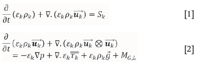
where k is the phase indicator, k = L for the liquid phase and k = G for the gas phase, ek is the volume fraction, /% is the phase density, and uk is the velocity of the k^thphase, while Sk is a mass source term. Mg,l is the interaction force between the phases, and epg is the gravity force, while = is the kth phase stress-strain tensor, given by:

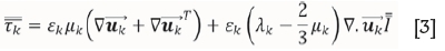
The volume fraction (or gas holdup) of the secondary phase was calculated from the mass conservation equations as:

where prG is the phase reference density, or volume-averaged density of the secondary phase in the solution domain. The volume fraction of the primary phase was calculated from the secondary phase one, since the sum of the volume fractions is equal to unity. The multiphase model was implemented and solved using the CFD code ANSYS FLUENT 14.5.

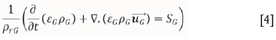
Interphase force

The interaction force between the two phases was modelled through the drag force incorporated into the multiphase model. The drag force per unit volume for bubbles in a swarm is generally presented as:

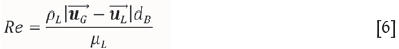
where C_Dis the drag coefficient, d_Bis the bubble diameter, and is the slip velocity. There are a number of empirical correlations that can be used to calculate the drag coefficient, Cd. The drag coefficient is normally presented in these correlations as a function of the bubble Reynolds number (Re), defined as:

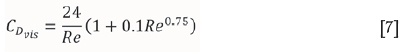
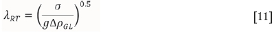
In the present study, the drag coefficient was calculated using the universal drag laws. In this case, the drag coefficient is defined in different ways depending on whether the prevailing regime is in the viscous regime category, the distorted bubble regime, or the strongly deformed capped bubbles regime. The different regimes are defined on the basis of the Reynolds number (Kolev, 2005). The subsequent expressions for the drag coefficient are derived from single-bubble equations, which are then modified to account for bubble swarm effects. In the viscous regime the drag coefficient is presented as:

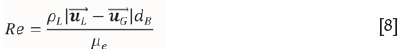
where Re is the relative Reynolds number for the primary phase L and the secondary phase G defined as:

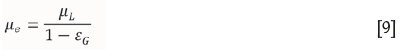
and μe is the effective viscosity for the bubble-liquid mixture given by:

In the distorted bubble regime the drag coefficient is given as follows:

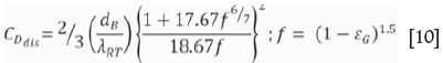
where λ_rt is the Rayleigh-Taylor instability wavelength, defined as:

and σ is the surface tension, g the gravitational acceleration, and ΔpGL is the absolute value of the density difference between the phases G and L.

For the strongly deformed, capped bubbles regime, the following drag coefficient is used:

Under churn-turbulent flow conditions, the drag coefficient is calculated using Equation [12]. Further details about the universal drag laws are available in a recent multiphase flow dynamics book (Kolev, 2005).

Turbulence modelling

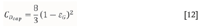
Turbulence in the continuous phase was modelled using the k-ε realizable turbulence model, a RANS (Reynolds-Averaged Navier-Stokes)-based model in which the time-averaged Navier-Stokes (RANS) equations are solved in place of the instantaneous Navier-Stokes equations to produce a time-averaged flow field. Alternative turbulence modelling approaches such as direct numerical simulation (DNS) or large-eddy simulation (LES) would require very dense computational grids and small time-steps, with subsequent increase in the computational effort required for the simulations. These methods are therefore not available when using the E-E multiphase model in ANSYS FLUENT. The averaging procedure introduces additional unknown terms; the Reynolds stresses, which are subsequently resolved by employing Boussinesq's eddy viscosity concept where the Reynolds stresses (or turbulent stresses) are related to the velocity gradients according to the following equation:

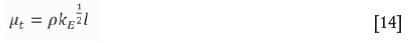
where μ_t is the turbulent or eddy viscosity, is the turbulent kinetic energy, and by is the Kronecker delta. The Kronecker delta is important in order to make the eddy viscosity concept applicable to normal stresses where i = y.

The turbulent viscosity is in turn related to a velocity scale and a length scale of the turbulence according to the Prandtl-Kolmogorov formula, which can be written as:

The velocity scale is calculated from the turbulent kinetic energy (kE) equation, while the length scale is obtained from the turbulent dissipation (ε) equation. The k-ε model is therefore a two-equation model in which two separate transport equations are solved to determine the velocity scale and the length scale of the turbulent motion. Turbulence in the near-wall region was modelled using standard wall functions to calculate turbulence quantities in the region near to the walls of the column.

Geometry and mesh

For the purposes of the present research, the model considers only the collection zone of the flotation column. Therefore the froth zone was not included in the model. A further simplification was achieved by leaving the sparger out of the model geometry. Instead, the air was introduced from the bottom part of the column over the entire column cross-section. This will not affect the required gas holdup prediction since the ratio of column cross-section to sparger surface area was about 1:1 in the experimental flotation column. The result of these simplifications is that the model geometry is reduced to a cylindrical vessel of height equal to the collection zone height (305 cm in this case) and diameter equal to the diameter of the experimental flotation column.

A mesh comprising mainly hexahedral elements was generated over the model geometry using the sweep method in ANSYS Meshing. Five mesh sizes were investigated in order to obtain grid-independent numerical results. The mesh sizes are summarized in Table I, together with their respective attributes.

 

 

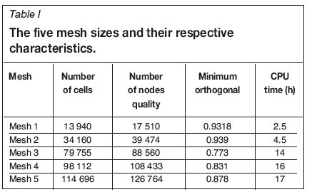
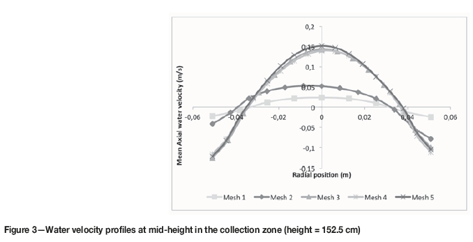
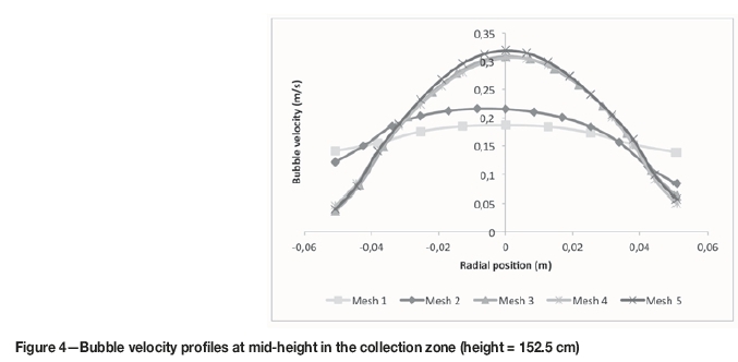
The axial water and bubble velocity profiles obtained for the different mesh sizes are shown in Figure 3 and Figure 4, respectively. Grid independence was achieved with mesh 3 to mesh 4 and 5. Mesh 3 (79 755 elements) was therefore selected for all subsequent simulations in this study.

Boundary conditions

Air bubbles were introduced into the column through mass and momentum source terms at the column bottom. The source terms were calculated from the respective superficial gas velocities and were applied over the entire column cross-section at the bottom (source) and at the top (sink) of the collection zone.

For the liquid phase, the top of the collection zone was modelled as a velocity inlet boundary where inlet velocity was specified as equal to superficial liquid velocity //. Since the computational domain being considered is the collection zone of the column, the superficial liquid velocity must include the feed rate plus the bias water resulting from wash water addition. The superficial liquid velocity is therefore equal to the superficial tailing rate, /.

The bottom part was also modelled as velocity inlet where exit velocity was set equal to minus superficial liquid velocity. At the column wall, no slip boundary conditions were applied for both the air bubbles and the liquid phase.

Numerical solution methods

The momentum and volume fraction equations were discretized using the first-order upwind scheme. The first-order upwind scheme was also employed for turbulence kinetic energy and dissipation rate discretization. A time step size of 0.05 seconds was used in all the simulations. The simulations were run up to a flow time of at least 240 seconds. Time averaging was carried out over the last 120 seconds.

 

Results and discussion

If the entire range of bubble sizes encompassing the different flow regimes is known, CFD simulations can be conducted for a range of superficial gas velocities covering the different flow regimes. A plot of gas holdup versus superficial gas velocity can then be used to determine the point of departure from bubbly flow conditions, as described earlier. For a system comprising water and air without frother, an empirical formula derived by Shen (1994) can be used to calculate the Sauter mean bubble size as a function of the superficial gas velocity. However, a similar empirical equation derived for column flotation conditions where frother plays an important role in determining the bubble size is limited to superficial gas velocities ranging from 1 to 3 cm/s. The first set of CFD results presented in this study is therefore obtained using bubble sizes calculated for a system without frother. The gas holdup versus superficial gas velocity relationship obtained is then used to delineate the different flow regimes prevailing in the column.

Once the flow regimes are identified, the evolution of radial gas holdup profiles and gas holdup versus time graphs can be examined for the flow regimes determined from the gas holdup versus superficial gas velocity graph. Radial gas holdup profiles and gas holdup versus time graphs are then used to determine the maximum superficial gas velocity for a column operating with an average bubble size of 1.5 mm, which is comparable with typical bubble sizes in industrial flotation columns. The radial gas holdup profiles were obtained at the mid-height position (152.5 cm height) in the column. On the other hand, the gas holdup versus time graphs were obtained from a surface monitor located at the column mid-height position, from which area-weighted average gas holdup measurements were recorded at 5-second intervals.

It is important at this stage to clarify the definition of regime transition and churn-turbulent flow regime as used in the present study. Churn-turbulent flow is normally associated with a wide bubble size distribution, including large bubbles. However, the CFD simulations in the present research were conducted with a single mean bubble size assigned for each superficial gas velocity. Furthermore, in order to investigate the flow regime transition for conditions relevant to column flotation, the other set of CFD simulations was performed with the bubble size held at a constant value of 1.5 mm while increasing the superficial gas velocity to determine the maximum superficial gas velocity for that particular bubble size. The reference to churn-turbulent flow in the present study is therefore not based on a wide bubble size distribution consisting of of large bubbles in the presence of smaller ones. On the other hand, a CFD model coupled with a bubble population balance model can be used to predict bubble size distributions in the column. However, bubble population balance modelling was beyond the scope of the present research. A possible alternative that can be used to simulate bubble size distributions is to apply a Eulerian-Lagrangian model. This approach was not applied in the present study due to its higher computational cost. A Eulerian-Lagrangian model would also require prior knowledge of the largest and smallest bubble sizes. This information was not readily available in the present research.

According to Lockett and Kirkpatrick (1975) there are three main reasons for breakaway from ideal bubbly flow: flooding, liquid circulation, and the presence of large bubbles. It should therefore be possible to identify regime transition from changes in the pattern and intensity of the liquid circulation in the column even if changes in bubble size are negligible or absent. However, the absence of large bubbles is likely to have an effect on the prediction of the location of the transition zone as well as on the shape of the radial gas holdup profile. On the other hand, the liquid circulation pattern and its intensity depend on the prevailing radial gas holdup profile in the column (Hills, 1974).

Saddle-shaped gas holdup profiles have already been related to bubbly flow conditions in two-phase flows (Kobayasi, Iida, and Kanegae, 1970; Serizawa, Kataoka, and Michiyoshi, 1975). However, the bubbly flow regime is generally characterized by a radially uniform gas holdup distribution (Ruzicka et at, 2001; Vial et al, 2001; Shaikh, and Al-Dahhan, 2007). Both saddle and flat gas holdup profiles can therefore be considered to indicate the existence of the bubbly flow regime in the column. On the other hand, the churn-turbulent flow regime is generally distinguished by a non-uniform radial gas holdup distribution causing bulk liquid circulation. Parabolic gas holdup profiles are therefore interpreted to signify churn-turbulent flow conditions in the column.

Water and air only (without frother)

For the water and air only (no frother) system, CFD simulations were carried out for superficial gas velocities ranging from 1.01 to 14 cm/s to encompass both the bubbly flow and churn-turbulent flow regimes. The Sauter mean bubble size for a multi-bubble system without frother (i.e., water and air only) can be calculated as a function of the superficial gas velocities from the following empirical formula (Shen, 1994):

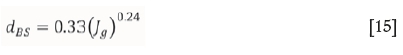
This empirical formula was derived for a laboratory flotation column with a porous stainless steel sparger similar to the one that was used in the column modelled in the present work. The equation was therefore used in the present work to calculate the average bubble sizes that were subsequently used in the CFD simulations.

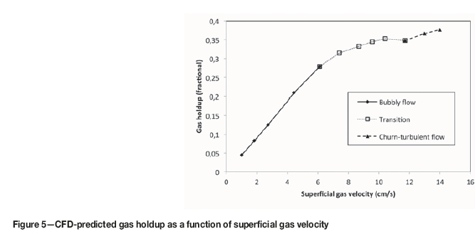
Gas holdup versus superficial gas velocity (gas rate) graph The graph of gas holdup versus superficial gas velocity obtained from CFD simulations is presented in Figure 5. The different flow regimes can be cleared delineated as follows:

► Bubbly flow regime; Jg 1.01-6.12 cm/s (linear portion of the graph)

► Transition; 6.12 <J_g< 11.71 cm/s (deviation from linear relationship between gas holdup and superficial gas velocity)

► Churn-turbulent flow; Jg > 11.71 cm/s (third portion of the gas holdup versus superficial gas velocity graph).

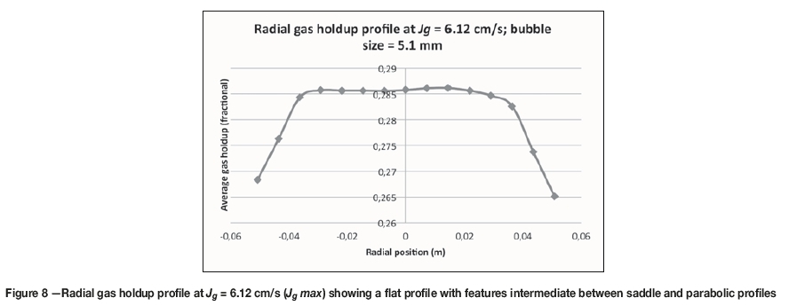
The maximum superficial gas velocity (Jg max) before loss of bubbly flow is therefore equal to 6.12 cm/s for the water and air only system without frother. This value compares well with the maximum superficial gas velocity of 5.25 cm/s for loss of bubbly flow predicted from drift flux theory by Xu, Finch, and Uribe-Salas (1991).

Having delineated the different flow regimes using the gas holdup versus superficial gas velocity relationship, the evolution of the radial gas holdup profiles was examined as the superficial gas velocity increased from 1.01 cm/s to 14 cm/s.

Radial gas holdup profiles

A number of different types of radial gas holdup profiles were obtained from the CFD simulations, including saddle-shaped, flat, and parabolic profiles. These profiles were then related to the flow regimes defined from the gas holdup/superficial gas velocity relationship (Figure 5).

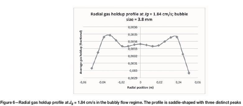
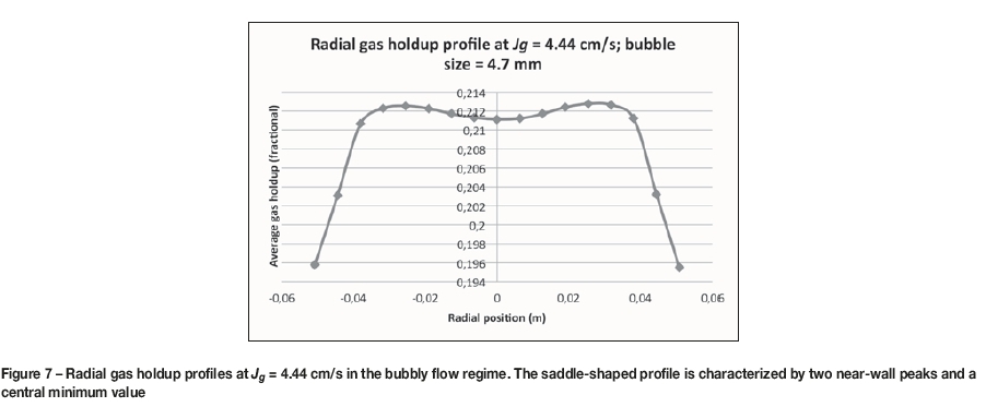
Three types of radial gas holdup profiles were observed in the bubbly flow regime. At the lower superficial gas velocities (Jg 1.01-2.73 cm/s), saddle-shaped profiles with three distinct peaks were observed with one peak at the centre and two other peaks located near the walls of the column, as shown in Figure 6 for Jg = 1.84 cm/s. The profiles then changed to ones with two near-wall peaks and a central minimum point as the superficial gas velocity increased to Jg = 4.44 cm/s, as illustrated in Figure 7. With further increase in the superficial gas velocity the central minimum point disappeared and the radial gas holdup profile became flat. The maximum superficial gas velocity Jg_max= 6.12 cm/s) before loss of bubbly flow is therefore characterized by a flat radial gas holdup profile with intermediate features between saddle and parabolic profiles, as shown in Figure 8.

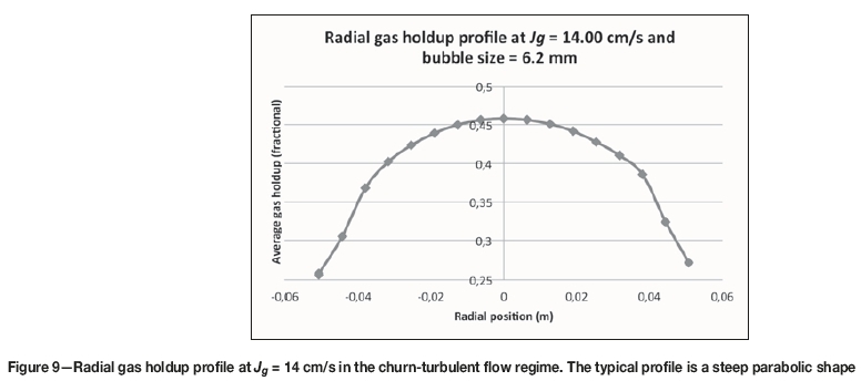
The transition from bubbly flow to churn-turbulent flow was gradual and characterized by flat (Jg = 7.41 cm/s) to parabolic (Jg 8.70-11.71 cm/s) radial gas holdup profiles. The parabolic profiles became progressively steeper as the superficial gas velocity increased. Eventually the flow regime changes into churn-turbulent flow (Jg > 11.71 cm/s), which is characterized by steep parabolic gas holdup profiles as shown in Figure 9.

Gas holdup versus time graphs

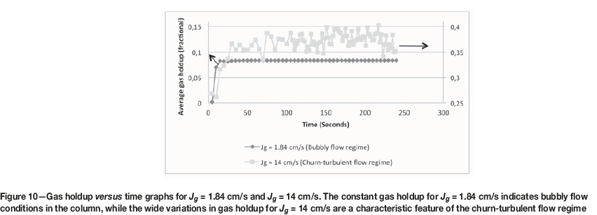
Another method that was used to distinguish flow regimes in the water-air system using CFD simulations was by means of gas holdup versus time graphs. The two extreme cases, bubbly flow and churn-turbulent flow, are compared in Figure 10. It can be seen that the gas holdup versus time was mostly constant in the bubbly flow regime (Jg = 1.84 cm/s), while very wide variations in gas holdup were observed in the churn-turbulent flow regime (i.e., Jg = 14 cm/s). The transition from bubbly flow to churn-turbulent flow pattern was gradual and characterized by moderate to large fluctuations in gas holdup, with the gas holdup variations becoming increasingly intense as the superficial gas velocity increased.

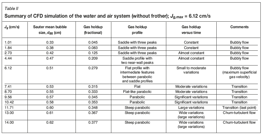
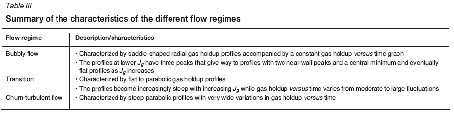
The results from the CFD simulations of the water and air only (no frother) system, where bubble sizes are calculated from the superficial gas velocity according to Equation [15], are summarized in Table II. The progression from bubbly flow conditions to churn-turbulent flow can also be clearly appreciated from this table. The distinguishing characteristics of the flow regimes are summarized in Table III.

Water with frother (as in column flotation)

In flotation columns, the bubble size depends not only on the superficial gas velocity, but also on other physical chemical characteristics of the gas-liquid system. In this case, the bubble size can be calculated as a function of the superficial gas velocity according to the following relationship (Finch and Dobby, 1990; Yianatos and Finch, 1990).

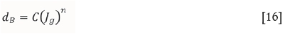
where C and n are constants. The constant C is a fitting parameter which depends mainly on frother concentration, the sparger size, and column size. Simulations were carried out for the experimental conditions used by Xu, Finch, and Uribe-Salas (1991) and Xu etal. (1989), particularly the case in which the frother concentration was 10 ppm. The value of C was therefore equal to unity while n was 0.25.

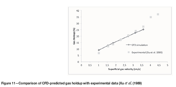
The gas holdup obtained from the CFD simulations is plotted as a function of superficial gas velocity in Figure 11. The experimental data from Xu et al. (1989) is included in the figure for comparison. It can be seen that the predicted gas holdup is in good agreement with the experimental data up to superficial gas velocity Jg = 3.60 cm/s. Above Jg = 3.60 cm/s, the relationship in Equation [16] is not applicable because the value of the exponent n (0.25) is valid for J_g1-3 cm/s (Yianatos and Finch, 1990). Unfortunately, there is no equation relating bubble size and superficial gas velocity for flow conditions above Jg = 3 cm/s. Therefore, the gas holdup versus superficial gas velocity graph obtained from CFD simulations cannot be used to determine the maximum superficial gas velocity since the range of bubble sizes for the different flow regimes cannot be completely determined.

Xu et al. (1989) used the gas holdup versus superficial gas velocity relationship to identify the maximum gas velocity for loss of bubbly flow. However, they reported a gradual and unclear transition from bubbly flow to churn-turbulent flow conditions. The maximum superficial gas velocity for conditions applicable in flotation columns can be obtained using radial gas holdup profiles and the gas holdup versus time graphs as already described. In this regard, CFD simulations are performed in the present study for a stipulated bubble size of 1.5 mm, which is similar to common bubble sizes used in column flotation. The bubble size is held constant during the simulations while increasing the superficial gas velocity to encompass both bubbly flow and churn-turbulent flow conditions.

Maximum superficial gas velocity for a column operating with 1.5 mm average bubble size

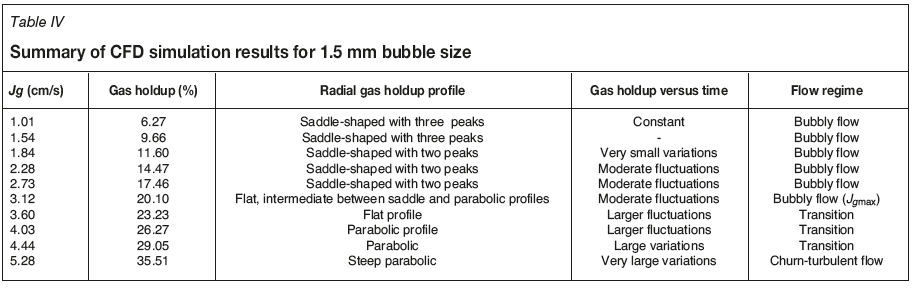
CFD simulations were performed with a constant bubble size of 1.5 mm for superficial gas velocities ranging from Jg = 1.01 to 6.12 cm/s. The liquid superficial velocity was maintained at Jl = 0.38 cm/s. Radial gas holdup profiles were examined for all the superficial gas velocities together with their corresponding gas holdup versus time plots.

Radial gas holdup profiles

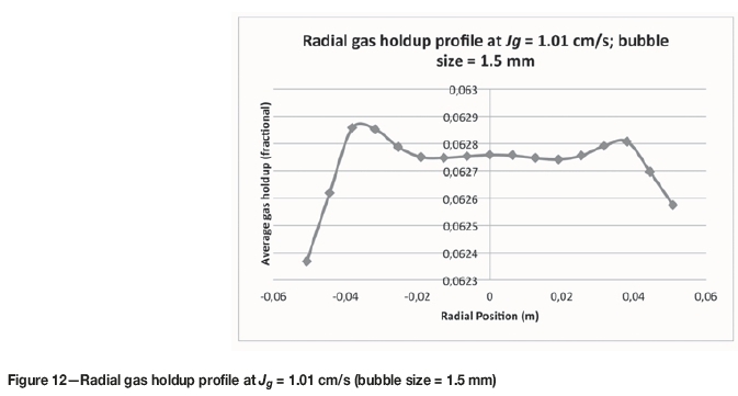
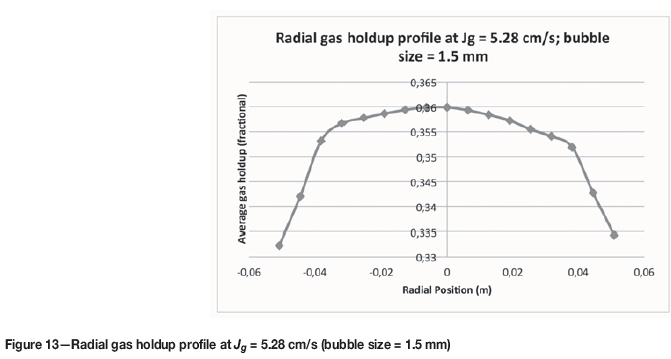
Saddle-shaped radial gas holdup profiles with three peaks were observed for Jg = 1.01 to 1.54 cm/s. The radial gas holdup profile for Jg 1.01 cm/s is presented in Figure 12 for elaboration. The profiles then changed to ones with two distinct peaks near to the column wall as Jg increased (Jg = 1.84 to 2.73 cm/s). On the other hand, a flat profile with intermediate features between saddle-shaped and parabolic profiles was observed for Jg = 3.12 cm/s. The column was therefore operating under bubbly flow conditions from Jg = 1.01 to 3.12 cm/s. In the churn-turbulent regime, steeper parabolic radial gas holdup profiles were observed from Jg= 5.28 cm/s, as shown in Figure 13.

Gas holdup versus time graphs

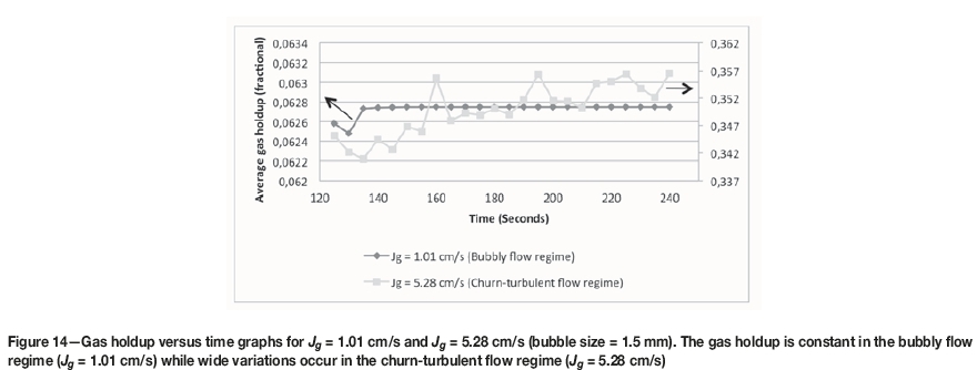
Gas holdup versus time graphs were used to confirm the existing flow regime in the column. A relatively constant gas holdup versus time was observed for Jg = 1.01 to 1.84 cm/s while moderate fluctuations in gas holdup were observed from Jg = 2.28 to 3.12 cm/s, confirming that the column was indeed in the bubbly flow regime in this range of superficial gas velocities. In contrast, very wide variations in gas holdup versus time were observed when the churn-turbulent flow regime prevailed in the column. The two extreme conditions, bubbly flow and churn-turbulent flow, are compared in Figure 14 for Jg= 1.01 cm/s and Jg= 5.28 cm/s.

Maximum (critical) superficial gas velocity

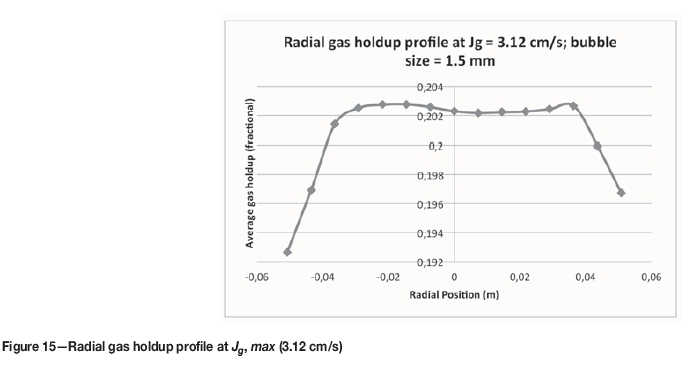
The maximum (critical) superficial gas velocity for transition into churn-turbulent flow was identified by the first appearance of flat radial gas holdup profiles with intermediate features between parabolic and saddle-shaped profiles at /g = 3.12 cm/s. The maximum superficial gas velocity (/g,_max) before loss of bubbly flow is therefore 3.12 cm/s for a flotation column operating with an average bubble size of 1.5 mm at superficial liquid velocity //) equal to 0.38 cm/s. This compares favourably with the maximum gas velocity of 3.60 cm/s reported by Xu, Finch, and Uribe-Salas (1991) and Xu et al. (1989) with reference to loss of interface. Indeed, these authors did report that loss of interface and loss of bubbly flow occurred at approximately the same superficial gas velocities. The predicted gas holdup at /g,max is equal to 20.1%, which compares favourably with the maximum gas holdup of 20 to 24% reported by Dobby, Amelunxen, and Finch (1985).

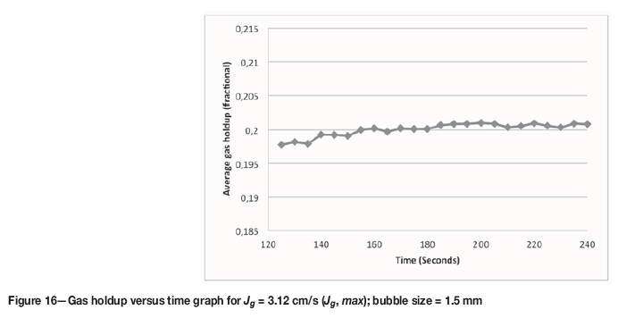
The radial gas holdup profile at Jg,max is shown in Figure 15, and its corresponding gas holdup versus time graph in Figure 16. It can be seen that the maximum superficial gas velocity is characterized by a flat gas holdup profile accompanied by moderate gas holdup fluctuations. The results from the CFD simulations for 1.5 mm bubble size are summarized in Table IV. The progression from bubbly flow conditions to churn-turbulent flow can be clearly seen in the table.

Liquid velocity vectors

Two different flow patterns were observed, depending on superficial gas velocity and bubble size. With increasing superficial gas velocity the well-known 'Gulf Stream' circulation pattern, in which the liquid rises in the centre of the column and descends near the column wall, was observed. In contrast, an 'inverse' circulation flow pattern, in which the liquid rises near the column wall but descends in the centre and immediately adjacent to the walls, occurred at lower superficial gas velocities. This is the first study to report such an inverse flow pattern in column flotation. However, similar flow reversals have been observed in experimental work on fluidized bed reactors (Lin, Chen, and Chao, 1985).

The inverse circulation pattern has been theoretically investigated in bubble columns and is associated with fully developed saddle-shaped radial gas holdup profiles (Clark, Atkinson, C., and Flemmer, 1987; Clark, van Egmond, and Nebiolo E. 1990). In the present study, the inverse circulation pattern was observed at /g = 1.01 cm/s and /g = 1.54 cm/s for simulations with bubble size = 1.5 mm and superficial liquid velocity = 0.38 cm/s. Saddle-shaped gas holdup profiles with two distinct peaks near the walls of the column were also present under these conditions. The liquid velocity vector plots obtained from CFD simulations are presented in Figure 17 and Figure 18 for the two circulation patterns.

 

 

 

 

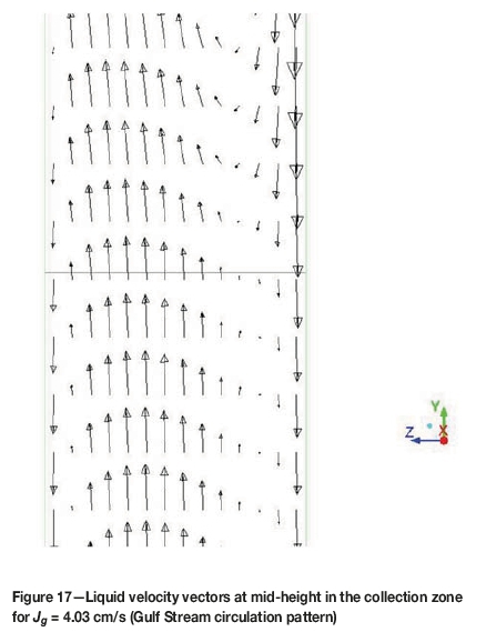
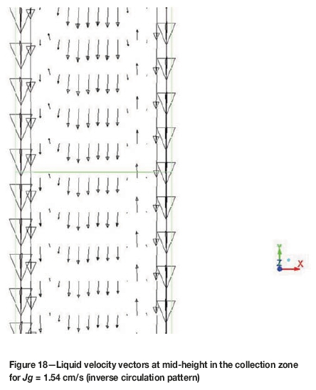
Clark, van Egmond, and Nebiolo (1990) have described the sequence of events that may initiate liquid circulation in bubble columns. In general, liquid circulation in bubble columns is initiated by density differences in the gas-liquid mixture, depending on the prevailing radial gas holdup profile. If the concentration of air bubbles is higher in the central part of the column compared to the outer annular region, the mean density of the mixture will be lower near the centre of the column than in the outer annulus. The hydrostatic pressure head will therefore be higher in the outer annulus, hence a radial pressure difference is set up inside the column. This will cause an inward radial movement of liquid and initiate liquid circulation. The inverse circulation pattern will occur if the concentration of bubbles is higher in the outer annular region, as in the case of saddle-shaped gas holdup profiles.

 

Conclusions

In this study, the evolution of the shape of the radial gas holdup profile in a pilot-scale flotation column was studied using CFD to delineate the maximum gas velocity for loss of bubbly flow. With increasing superficial gas velocity, the gas holdup profile passes through different stages, which can be used to define the prevailing flow regime in the column. The different flow regimes were also verified by the intensity of the local variations of the gas holdup.

In the bubbly flow regime, saddle-shaped and flat radial gas holdup profiles were obtained. These profiles were accompanied by minor to moderate gas holdup variations in the column. The transition regime was gradual and characterized by flat to parabolic gas holdup profiles. The parabolic profiles became progressively steeper as the superficial gas velocity increased. The corresponding gas holdup versus time graphs in the transition regime showed moderate to wide variations in gas holdup. On the other hand, the churn-turbulent flow regime was distinguished by steep parabolic gas holdup profiles with very wide variations in gas holdup versus time.

For conditions relevant to column flotation, the maximum superficial gas velocity was determined for a column operating with an average bubble size of 1.5 mm and superficial liquid velocity equal to 0.38 cm/s. The maximum superficial gas velocity was found to be equal to 3.12 cm/s. The corresponding maximum gas holdup value was 20.1%.

Two possible flow patterns were revealed in the simulated column in this study: the 'Gulf Stream' circulation pattern and an inverse circulation pattern. The latter was observed only in the presence of fully developed saddle-shaped radial gas holdup profiles.

The CFD simulations in the present study assumed a constant average bubble size for the flotation column. However, for the churn-turbulent regime, a bubble size distribution exists that could have an effect on the hydrodynamics of the column. CFD models coupled with a bubble population balance model should therefore be considered in future studies in order to account for bubble size distributions in the transition and churn-turbulent flow regimes.

 

Nomenclature

CD Drag coefficient, dimensionless

dB Bubble diameter, mm

dBS Sauter mean bubble size

Drag force per unit volume, N/m³

Gravitational acceleration, 9.81 m/s²

Jg Superficial gas velocity, cm/s

Jg,max Maximum superficial gas velocity

Jl Superficial liquid velocity

kE Turbulence kinetic energy, m²/s²

P Pressure, Pa

Re Reynolds number, dimensionless

Sk Mass source term for phase k, kg/m3-s

u Reynolds averaged velocity, m/s

u' Velocity fluctuation, m/s

Greek letters

εc Air volume fraction or gas holdup

ε Volume fraction

ε Turbulence dissipation rate, m2/s3

λrt Rayleigh-Taylor instability wavelength

μ Viscosity, kg/m-s

μί Turbulent viscosity, kg/m-s

ρ Density, kg/m³

σ Surface tension (N/m)

Viscous stress tensor, Pa

Subscripts

B Bubble

D Drag

G, g Gas

i, j Spatial directions

k Phase

L, l Liquid

 

Acknowledgements

The authors would like to acknowledge the Centre for International Cooperation at VU University Amsterdam (CIS-VU) and the Copperbelt University (CBU) for providing the scholarship and subsequent funding for this research through the Nuffic-HEART Project. We would also like to acknowledge the Process Engineering Department at Stellenbosch University for providing the necessary facilities that made this research possible. The CFD simulations in our studies were performed using the University of Stellenbosch's Rhasatsha High Performance Computing (HPC) cluster: http://www.sun.ac.za/hpc

 

References

Clark, N., Atkinson, C., and Flemmer, R. 1987. Turbulent circulation in bubble columns. AIChE Journal, vol. 33, no. 3. pp. 515-518.         [ Links ]

Clark, N., van Egmond, J., and Nebiolo E. 1990. The drift-flux model applied to bubble columns and low velocity flows. International Journal of Multiphase Flow, vol. 16, no. 2. pp. 261-279.         [ Links ]

Dobby, G., Amelunxen, R., and Finch, J. 1985. Column flotation: Some plant experience and model development. Proceedings of the First IFAC Symposium on Automation/or Mineral Resource Development, Brisbane, Australia, 9-11 July. IFAC Proceedings, vol. 18, no. 6. pp. 259-263.         [ Links ]

Finch, J.A. and Dobby, G.S. 1990. Column Flotation. Pergamon, Oxford, UK.         [ Links ]

Hills, J. 1974. Radial non-uniformity of velocity and voidage in a bubble column. Transactions of the Institution of Chemical Engineers, vol. 52, no. 1. pp. 1-9.         [ Links ]

Ityokumbul, M. 1992. A new modelling approach to flotation column desing . Minerals Engineering, vol. 5, no. 6. pp. 685-693.         [ Links ]

Kobayasi, K., Iida, Y., and Kanegae, N. 1970. Distribution of local void fraction of air-water two-phase flow in a vertical channel. Bulletin of JSME, vol. 13, no. 62. pp. 1005-1012.         [ Links ]

Kolev, N.I. 2005. Multiphase Flow Dynamics 2: Thermal and Mechanical Interactions. 2nd edn. Vol. 2. Springer, Berlin, Germany.         [ Links ]

Langberg, D. and Jameson, G. 1992. The coexistence of the froth and liquid phases in a flotation column. Chemical Engineering Science, vol. 47, no. 17. pp. 345-355.         [ Links ]

Lin. J., Chen, M., and Chao, B. 1985. A novel radioactive particle tracking facility for measurement of solids motion in gas fluidized beds. AIChE Journal, vol. 31, no. 3. pp. 465-73.         [ Links ]

Lockett, M. and Kirkpatrick, R. 1975. Ideal bubbly flow and actual flow in bubble columns. Transactions of the Institution of Chemical Engineers, vol. 53. pp. 267-273.         [ Links ]

Mecklenburg, M.M. 1992. Hydrodynamic study of a downwards concurrent bubble column. MEng dissertation, McGill University, Montreal, Canada.         [ Links ]

Ruzicka, M., Zahradnik, J., DrahoS, J., and Thomas N. 2001. Homogeneous-heterogeneous regime transition in bubble columns. Chemical Engineering Science, vol. 56, no. 15. pp. 4609-4626.         [ Links ]

Serizawa, Α., Kataoka, I., and Michiyoshi, 1.1975. Turbulence structure of air-water bubbly flow - II. local properties. International Journal of Multiphase Flow, vol. 2, no. 3. pp. 235-246.         [ Links ]

Shaikh, Α. and Al-Dahhan, M.H. 2007. Α review on flow regime transition in bubble columns. International Journal of Chemical Reactor Engineering, vol. 5, no. 1. https://doi.org/10.2202/1542-6580.1368        [ Links ]

Shen, G. 1994. Bubble swarm velocities in a flotation column. PhD dissertation, McGill University; Montreal, Canada.         [ Links ]

Summers, A.J. 1995. Α study of the operating variables of the Jameson cell. MEng dissertation, McGill University, Montreal, Canada.         [ Links ]

Vial, C., Poncin, S., Wild, G., and Midoux, N. 2001. Α simple method for regime identification and flow characterisation in bubble columns and airlift reactors. Chemical Engineering and Processing: Process Intensification, vol. 40, no. 2. pp. 135-151.         [ Links ]

Xu, M., Finch, J., and Uribe-Salas, Α. 1991. Maximum gas and bubble surface rates in flotation columns. International Journal of Mineral Processing, vol. 32, no. 3. pp. 233-250.         [ Links ]

Xu, M., Uribe-Salas, Α., Finch, J., and Gomez, C. 1989. Gas rate limitation in column flotation. Processing of Complex Ores: Proceedings of the International Symposium on Processing of Complex Ores, Halifax, Nova Scotia, 20-24 August 1989. Elsevier. pp. 397-407.         [ Links ]

Yianatos, J. and Finch, J. 1990. Gas holdup versus gas rate in the bubbly regime. International Journal of Mineral Processing, vol. 29, no. 1. pp.141-146.         [ Links ] ♦

 

 

Paper received Sep. 2017
Revised paper received Jun. 2018.