PAPERS OF GENERAL INTEREST

 

Prediction of gas holdup in a column flotation cell using computational fluid dynamics (CFD)

 

 

I. Mwandawande^I; G. Akdogan^I; S.M. Bradshaw^I; M. Karimi^II; N. Snyders^I

^IUniversity of'Stellenbosch, South Africa
^IIChalmers University of Technology, Gothenburg, Sweden

 

 

---

SYNOPSIS

Computational fluid dynamics (CFD) was applied to predict the average gas holdup and the axial gas holdup variation in a 13.5 m high cylindrical column 0.91 m diameter. The column was operating in batch mode. A Eulerian-Eulerian multiphase approach with appropriate interphase momentum exchange terms was applied to simulate the gas-liquid flow inside the column. Turbulence in the continuous phase was modelled using the k-e realizable turbulence model. The predicted average gas holdup values were in good agreement with experimental data. The axial gas holdup prediction was generally good for the middle and top parts of the column, but was over-predicted for the bottom part of the column. Bubble velocity profiles were observed in which the axial velocity of the air bubbles decreased with height in the column. This may be related to the upward increase in gas holdup in the column. Simulations were also conducted to compare the gas holdup predicted with the universal, the Schiller-Naumann, and the Morsi-Alexander drag models. The gas holdup predictions for the three drag models were not significantly different.

Keywords: column flotation, computational fluid dynamics (CFD), gas holdup.

---

 

 

Introduction

Column flotation is an important concentration technology that is used in the mineral processing and coal beneficiation industries. The growing interest in the use of column flotation in mineral processing has been attributed to the simpler flotation circuits and improved metallurgical performance compared to conventional flotation cells (Finch and Dobby, 1990). Flotation columns have also found other applications outside mineral processing, such as de-inking of recycled paper (Finch and Hardie, 1999).

In column flotation, a rising swarm of air bubbles generated by means of air spargers is employed to collect the valuable mineral particles and separate them from the gangue minerals in a countercurrent process. Wash water, which is continuously fed at the top of the column, is used to eliminate entrained particles and stabilize the froth. The column volume can be divided into two sections - the collection zone in which the bubbles collect the floatable mineral particles, and the cleaning zone (or froth zone) where product upgrading is enhanced through the removal of unwanted particles entrained in the water mixed with bubbles from the collection zone.

One of the most important operational variables affecting the metallurgical performance of flotation columns is gas holdup in the collection zone (Gomez et al., 1991). Gas holdup is defined as the volumetric fraction (or percentage) occupied by gas at any point in a column (Finch and Dobby, 1990). Some studies have reported that gas holdup affected both the recovery and grade in industrial and pilot-scale flotation columns (Leichtle, 1998; López-Saucedo et al., 2012). These studies reported a linear relationship between gas holdup and recovery. Linear relationships between gas holdup and the flotation rate constant have also been identified, highlighting its effect on flotation kinetics (Hernandez, Gomez, and Finch, 2003; Massinaei et al., 2009). On the other hand, other researchers have suggested that gas holdup could be used for control purposes in column flotation (Dobby, Amelunxen, and Finch, 1985). However, apart from its potential in control, gas holdup also has diagnostic applications, for example the sudden drop in gas holdup that occurs when a sparger is malfunctioning.

Because of its importance in column flotation, gas holdup has been studied by several researchers who have reported average and local gas holdup measurements in the column (Gomez et al., 1991, 1995; Paleari, Xu, and Finch, 1994; Tavera, Escudero, and Finch, 2001). Computational fluid dynamics (CFD) has emerged as a numerical modelling tool that can be used to enhance the understanding of the complex hydrodynamics pertaining to flotation cells (Deng, Mehta, and Warren, 1996; Koh et al., 2003; Koh and Schwarz, 2009; Chakraborty, Guha, and Banerjee, 2009). For column flotation cells, CFD modelling has been applied to predict the average gas holdup for the whole column (Koh and Schwarz, 2009; Chakraborty, Guha, and Banerjee, 2009). However, the gas holdup has been observed to vary with height along the collection zone of the flotation column (Gomez et al., 1991, 1995; Yianatos et al., 1995), increasing by almost 100% from the bottom to the top of the column. The increase in gas holdup with height is attributed to the hydrostatic expansion of bubbles (Yianatos et al., 1995; Zhou and Egiebor, 1993).

Despite the reported increase in gas holdup along the column height, the CFD literature on column flotation does not account for this phenomenon. This could result in the under-prediction of gas holdup, particularly in cases where the available experimental measurements were taken near the top of the column. For example, Koh and Schwarz (2009) reported an average gas holdup of 0.176 for the whole column compared with 0.23 measured at the top part of the column. The height of this column was 4.9 m. Industrial flotation columns are typically 9-15 m high (Finch and Dobby, 1990). This highlights the significance of considering the axial gas holdup variation in column flotation CFD models.

The aim of the present work was therefore to investigate the application of CFD for predicting not only the average gas holdup, but also the axial gas holdup variation in the column. In this regard, CFD was used to model a cylindrical pilot column that was used in previous studies on axial gas holdup distribution (Gomez et al., 1991, 1995). Since the corresponding experimental work was performed in two-phase systems with water and air only (in the presence of a frother), two-phase simulations were conducted in the present study in order to simulate the actual conditions in the pilot column.

In an attempt to understand the observed axial variations in gas holdup, Sam. Gomez, and Finch (1996) conducted experiments in which axial velocity profiles of single bubbles were measured. However, column flotation involves a swarm of bubbles as opposed to single bubbles. Swarms of moving bubbles are known to have velocities that are different from those derived for the case of single bubbles (Gal-Or and Waslo, 1968; Delnoij, Kuipers, and van Swaaij, 1997). CFD is capable of predicting the entire flow fields of the various phases involved in the flotation process. For this reason, CFD is a suitable tool that can be used to simulate the axial variation in bubble velocity in order to understand the spatial gas holdup distribution in the column. Axial bubble velocity profiles are therefore included in this study in the context of their possible relationship with the axial gas holdup profile along the column height.

 

Description of the column

The pilot flotation column was used in previous research (Gomez et al., 1991, 1995) to study gas holdup in the collection zone. It has a diameter of 0.91 m and a height of approximately 13.5 m. The experimental work was conducted with air and water only in a batch process. Air was introduced into the column through three Cominco-type spargers.

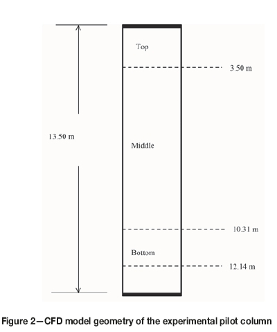
This column was selected for the present CFD modelling studies because axial gas holdup variation had been earlier identified and investigated for the column. The gas holdup data available for the column was therefore used to validate the CFD results in the present work. In the experimental work (Gomez et al., 1991, 1995), the column was divided into three sections over which pressure measurements were taken. An illustration of the column is provided in Figure 1 to show the position of the pressure sensing devices and their respective distances from the top of the column.

 

 

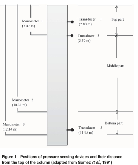
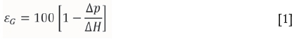
For the air-water system the gas holdup can be determined from the pressure difference Δp between two points separated by a distance ΔΗ according to the following equation (Gomez et al., 1991:

The gas holdup in the experimental work was therefore calculated from pressure measurements taken over the three sections using pressure transducer 2 for the top part, water manometers 1 and 2 for the middle part, and water manometers 2 and 3 for the bottom part. The average gas holdup for the whole column was calculated using the readings from pressure transducer 3.

The experimental measurements were conducted for superficial gas velocities Jg) of 0.72, 0.93, 1.22, 1.51, 1.67, 2.23, and 2.59 cm/s. Superficial gas velocity is defined as the volumetric flow rate of gas divided by the column cross-sectional area (Finch and Dobby, 1990) and is measured in cm/s.

 

CFD model description

Multiphase model

A two-fluid model has been recommended for studying large-scale flow structures in pilot- and industrial-scale bubble columns, due to its relatively low computational cost (Delnoij, Kuipers, and van Swaaij, 1997). A Eulerian-Eulerian two-fluid model was therefore selected in the present research, considering the large size of the pilot flotation column that was to be modelled. Subsequent CFD simulations in this study were performed using the Ansys Fluent 14.5 software package.

In the Eulerian-Eulerian approach the different phases are considered separately as interpenetrating continua. Momentum and mass conservation equations are then solved for each of the phases separately. Interaction between the phases is generally accounted for through inclusion of the drag force, while other forces such as the virtual mass and lift force can be neglected (Chen, Sanyal, and Dudukovic, 2004; Chen, Dudukovic, and Sanyal, 2005; Chen et al., 2009). Momentum exchange between the phases in this study was therefore accounted for by means of the drag force only. Since there is no mass transfer between the phases, the Reynolds -averaged mass and momentum equations are given as:

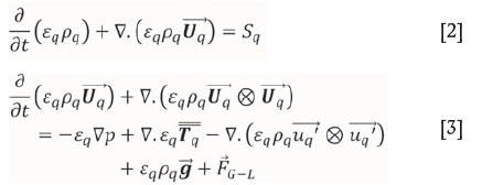
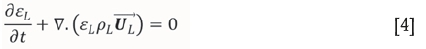
where q is the phase indicator, q = L for the liquid phase and q = G for the gas phase, εq is the volume fraction, pq is the phase density, and (Üq ) is the Reynolds-averaged velocity of the q^thphase, while Sq is the mass source term, F_G-Lis the interaction force between the phases, and eqpqg is the gravity force. Closure relations are required in order to close the Reynolds stress tensor which arises from the velocity fluctuations u'. The liquid phase was modelled as incompressible, hence its continuity (mass conservation) equation is simplified as follows:

In the present study, water was modelled as the continuous phase (primary phase) while air bubbles were treated as a secondary phase which is dispersed in the continuous phase. The volume fraction (or gas holdup) of the secondary phase was calculated from the mass conservation equations as:

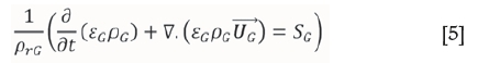
where prG is the volume-averaged density of the secondary phase in the computational domain. The volume fraction of the primary phase was calculated from that of the secondary phase, considering that the sum of the volume fractions is equal to unity.

In order to obtain the correct local distribution of the gas phase, previous researchers implemented compressibility effects in their CFD models using the ideal gas law (Schallenberg, Enß, and Hempel, 2005; Michele and Hempel, 2002). Similarly, the axial gas holdup variation in the present study was incorporated in the CFD simulations by applying

the ideal gas law to compute the density of the secondary phase (pg) as a function of the local pressure distribution in the column according to the following equation:

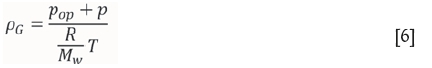
where ρ is the local relative (or gauge) pressure predicted by CFD, pop is operating pressure, R is the universal gas constant, M_wis the molecular weight of the gas, and T is temperature.

Drag force formulations

Generally, the drag force per unit volume for bubbles in a swarm is given by:

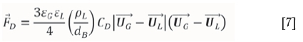
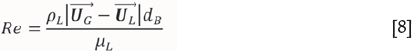
where C_Dis the drag coefficient, d_Bis the bubble diameter, and U_G- U_Lis the slip velocity. There are several empirical correlations for the drag coefficient, Cd, in the literature. The drag coefficient is normally presented in these correlations as a function of the bubble Reynolds number (Re). A constant value of the drag coefficient may also be used (Pfleger et al., 1999; Pfleger and Becker, 2001). The bubble Reynolds number is defined as:

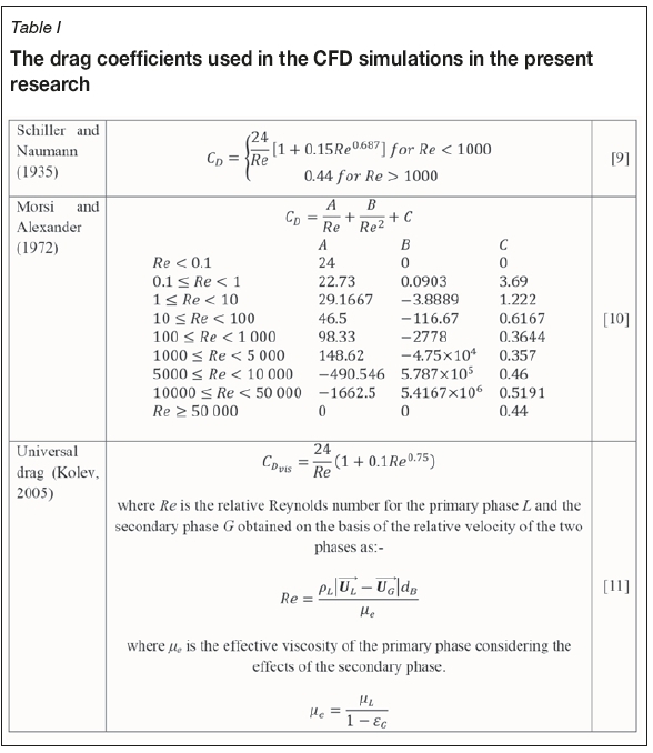
In the present research, simulations were carried out with three different drag coefficients. The first set of simulations was performed using the universal drag coefficient (Kolev, 2005). Subsequent simulations were conducted with the Schiller-Naumann (Schiller and Naumann, 1935) and Morsi-Alexander (Morsi and Alexander, 1972) drag coefficients in order to compare the suitability of the three drag models for the average and axial gas holdup computation in the flotation column. The equations describing the three drag coefficients are outlined in Table I.

The universal drag coefficient is defined differently for flows that are categorized as either in the viscous regime, the distorted bubble regime, or the strongly deformed capped bubbles regime, as determined by the Reynolds number. At the moderate superficial gas velocities simulated in this study, the viscous regime conditions apply. The equation presented in Table I is the one that is applicable when the prevailing flow is in the viscous regime. Further details about the universal drag laws are available in a recent multiphase flow dynamics book (Kolev, 2005).

Turbulence model

Turbulence was modelled using the realizable k-e turbulence model (Shih et al., 1995) which is a RANS (Reynolds-Averaged Navier-Stokes) based model. In the RANS modelling approach, the instantaneous Navier-Stokes equations are replaced with the time-averaged Navier-Stokes (RANS) equations, which are solved to produce a time-averaged flow field. The averaging procedure introduces additional unknowns; the Reynolds stresses. The Reynolds stresses are subsequently resolved by employing Boussinesq's eddy viscosity concept, where the Reynolds stresses (or turbulent stresses) are related to the velocity gradients according to the following equation:

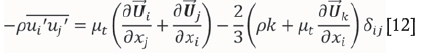
where u is the eddy or turbulent viscosity, k is the turbulence kinetic energy, and δ_ij is the Kronecker delta. The turbulent viscosity is then calculated from the turbulence kinetic energy (k) and the turbulence dissipation rate (ε). The Reynolds stresses are formulated based on the turbulent kinetic energy and shear stresses, which leads to better understanding of the flow characteristics of the column. The main difference between the standard k-ε turbulence model and the realizable version of this turbulence model is due to the different expression for the turbulent viscosity and an enhanced transport equation for the dissipation rate of turbulence, ε. The k-ε model is therefore a two-equation turbulence model, since two additional transport equations must be solved for the turbulence kinetic energy (k) and dissipation rates (ε). The differences between the realizable and the standard k-ε model would be more substantial where the flow includes strong vortices and rotation, such as in column flotation. Due to the abovementioned reasons, as well as preliminary studies of the turbulence models for the system under investigation, the realizable version of k-ε model was applied in this study. For the realizable k-ε model, the turbulence kinetic energy (k) and turbulence dissipation rate equations can be found elsewhere (Shih et al., 1995).

Boundary conditions

The sparging of gas into the column was modelled using source terms introduced in the gas-phase continuity equations for the computational cells at the bottom of the column. The gas phase is assumed to enter the column as air bubbles. Cominco spargers like those that were used in the simulated column are known for their uniform bubble distribution over the entire column cross-section (Paleari, Xu, and Finch, 1994; Harach, Redfearn, and Waites, 1990; Xu, Finch, and Huls, 1992). The air bubbles were therefore introduced over the entire column cross-section in the CFD model without including the physical spargers in the model geometry. The top of the column was modelled as a sink to simulate the exit of the air bubbles at the top of the collection zone. The mass and momentum source terms were calculated from the superficial gas (air) velocity, Jg, as follows:

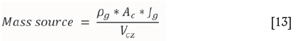
where pg is the density of air (1.225 kg/m3), Ac is the column cross-sectional area (m2), Jg is the superficial gas (air) velocity (m/s), and V_czis the volume of the cell zone where the source terms are applied. The momentum source terms were calculated from the respective mass source terms according to the following equation:

For the batch-operated column, there are no inlets or outlets for the liquid phase in the model. Boundary conditions were therefore specified for the column wall only. In this case, no slip boundary conditions were applied at the column wall for both the primary phase (water) and the secondary phase (air bubbles). The application of a source term of the sparger has been proven to be computationally affordable; moreover, it helps to introduce the gas bubbles in a uniform fashion across the column. The no-slip boundary condition for the column walls is a very well-established boundary condition that assumes that the fluid has zero velocity relative to the column wall.

Model geometry and mesh

A CFD model (geometry) of this column was subsequently developed considering the three sections as shown in Figure 2. Three-dimensional (3D) simulations of the cylindrical column were then conducted for five different superficial gas velocities, Jg, from 0.72 to 1.67 cm/s.

 

 

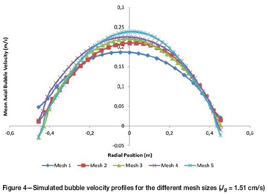
The meshing application of ANSYS Workbench was used to generate the mesh over the model geometry. The mesh was generated using the Sweep method, which creates a mesh comprising mainly hexahedral elements. Grid-dependency studies were conducted in order to eliminate the possibility of errors resulting from an unsuitable mesh size. The mesh was therefore progressively refined from an initially coarse mesh of cell size equal to 5 cm and number of cells equal to 97 188 until there were no significant changes in the simulated axial water and bubble velocity profiles.

The different mesh sizes that were investigated are presented in Table II, while the axial velocity profiles obtained for these meshes are shown in Figure 3 and Figure 4. It can be seen that the mean axial water and bubble velocity profiles do not change significantly from mesh 3 up to mesh 5. However, the axial velocity for mesh 5 is slightly higher than for mesh 3 and mesh 4. Therefore, based on these results mesh 4, comprising 884 601 elements with cell size equal to 2.25 cm, was used for all subsequent simulations, since it represented a reasonable trade-off between the required accuracy and the computational time for the simulations. A minimum orthogonal quality of 0.840 was obtained for the mesh.

 

 

Numerical solution methods

Momentum and volume fraction equations were discretized using the QUICK scheme, while First Order Upwind was employed for turbulence kinetic energy and dissipation rate discretization. The QUICK scheme provides up to third-order accuracy in the computations, while First Order Upwind is easier to converge. The time step size was 0.05 seconds.

For simulations that were difficult to converge the First Order Upwind scheme was used in place of the QUICK scheme until convergence. In some of such cases the time step size was changed from 0.05 seconds to 0.025 seconds to enhance convergence. The simulations were run up to flow times of between 400 seconds and 540 seconds since the bubble residence time in a similar sized column was measured at 4-5 minutes (Yianatos et al., 1994).

 

Results and discussion

Two sets of CFD simulations were carried out in this study to predict the average gas holdup and the axial gas holdup variation in the flotation column. The first set of simulations was conducted using the universal drag coefficient to calculate the drag force between the air bubbles and the liquid. Another set of simulations was then performed with the Schiller-Naumann and the Morsi-Alexander drag coefficients in order to compare the suitability of the different drag models for predicting gas holdup in the column. The simulation results obtained with the universal drag coefficient are presented first, followed by a comparison of the results obtained with the three different drag coefficients.

Simulation results with universal drag coefficient

Liquid flow field

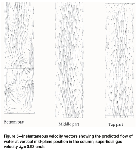
Figure 5 shows the predicted instantaneous velocity vectors of the liquid (water) at the vertical mid-plane position in the column. The liquid velocity field shows a typical circulating flow in the column in which the liquid is rising in the centre and descending near the walls of the column. This compares well with earlier CFD predictions for flotation columns (Deng, Mehta, and Warren, 1996; Koh and Schwarz, 2009), as well as experimental data on bubble columns (Hills, 1974; Devanathan, Moslemian, and Dudukovic, 1990). The type of liquid circulation where upward flow exists in the centre while downward flow prevails near the column walls is referred to as 'Gulf-Stream circulation' (Freedman and Davidson, 1969). The liquid circulation is intimately related to non-uniform radial gas holdup profiles in the column (Hills, 1974; Freedman and Davidson, 1969). This is because the density difference produced by non-uniform radial gas holdup profiles provides the driving force for the liquid circulation in the column. Non-uniform gas holdup profiles result in density differences, which will cause differences in pressure across the column. The liquid will then circulate in the direction of this pressure difference (Freedman and Davidson, 1969).

 

 

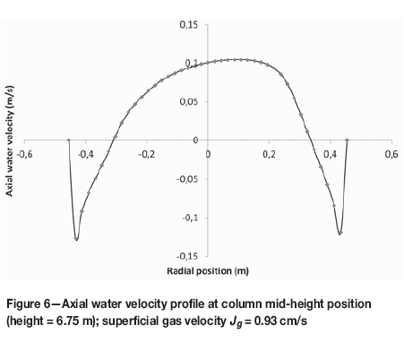
The simulated axial velocity profile of water at mid-height position in the column at time 540 seconds is presented in Figure 6. It can be seen that the water velocity is positive (upward) in the centre of the column and negative (downward) near the wall, hence confirming the circulation pattern in the column. The axial water velocity profile shown in Figure 6 is asymmetrical. Asymmetrical velocity profiles have also been reported by other researchers who conducted experimental studies on bubble columns (Devanathan, Moslemian, and Dudukovic, 1990).

 

 

Gas holdup distribution in the column

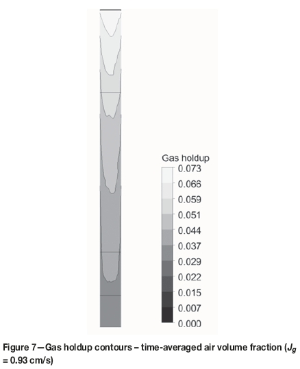
Figure 7 shows the time-averaged air volume fraction (gas holdup) contours in the column obtained from the CFD simulations. The gas holdup increases from the bottom to the top of the column, the holdup at the top being almost twice that at the bottom of the column. The axial increase in gas holdup has been attributed to the hydrostatic expansion of bubbles due to the decrease in hydrostatic pressure (Yianatos et al., 1995; Schallenberg, Enß, and Hempel, 2005). In the CFD simulations, the increase in gas holdup with increasing height in the column is achieved by applying the ideal gas model to compute the density of the air bubbles as a function of the predicted pressure field. Figure 7 also shows a radial variation in gas holdup, where the highest gas holdup occurs at the centre of the column.

 

 

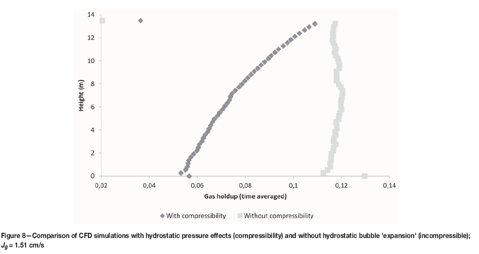
The CFD model was further tested for the case in which the effect of the hydrostatic pressure is neglected. In this case, the air bubbles were assigned a constant density of 1.225 kg/m³. The simulation results in which the air bubbles were modelled as incompressible (without hydrostatic 'expansion') were compared with the results in which compressibility effects are accounted for using the ideal gas law. This was done in order to determine whether there was no other source of change in axial gas holdup. The axial gas holdup profiles of the two cases are compared in Figure 8. The case with compressibility effects shows an axial gas holdup profile in which the gas holdup increases by at least 100% from bottom to top along the height of the column. On the other hand, the incompressible case does not show a significant increase in axial gas holdup. The decreasing hydrostatic pressure therefore plays the major role in creating an axial gas holdup profile in flotation columns.

Comparison of predicted gas holdup with experimental data

The gas holdup was obtained from CFD simulations as a volume-weighted average volume fraction of the air bubbles (or the average volume fraction over the whole volume). The predicted average gas holdup for the whole column is therefore the net volume-weighted average volume fraction for the three sections (bottom, middle, and top) of the column, while axial gas holdup was determined from the local value of air volume fraction in each of the three sections.

Figure 9 is a parity plot comparing the simulated (predicted) average gas holdup against the experimental gas holdup measurements (Gomez et al., 1991). The CFD predictions seem to be in good agreement with the experimental data.

The axial gas holdup predicted for each of the three sections (bottom, middle, and top) of the column is also compared against experimental data in Figures 10-13. The increase of gas holdup along the column height can be observed both in the CFD predictions and the experimental data. The axial gas holdup prediction for the middle part of the column gave an excellent comparison with experimental data, while that in the top part was slightly under-predicted for the higher superficial gas velocities (Jg = 1.51 cm/s and 1.67 cm/s).

 

 

 

 

 

 

 

 

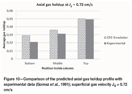
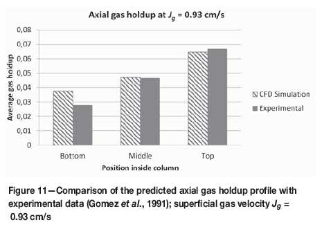
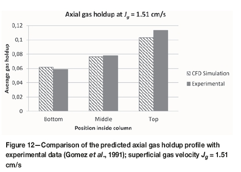
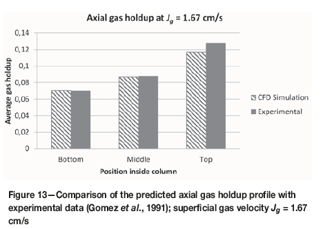
On the other hand, it can be observed from Figures 10-13 that the axial gas holdup is over-predicted for the bottom part of the column, especially at lower superficial gas velocities (Jg = 0.72 and 0.93 cm/s). This may be because the CFD model applies a constant bubble size of 1 mm and does not account for bubble coalescence and breakup in the column. When bubble coalescence and breakup are significant, the bubble size distribution in the column will be determined by the relative magnitudes of bubble coalescence and breakup (Bhole, Joshi, and Ramkrishna, 2008). At lower superficial gas velocities bubble coalescence will be the dominant process (Prince and Blanch, 1990), hence the experimental gas holdup in the bottom part of the column will be lower than the predicted value if the resulting average bubble size is larger than the 1 mm that was used in the simulations. However, with increasing superficial gas velocity bubble breakup reduces the average bubble size to around the 1 mm value used in the simulations, hence the observed improvement in axial gas holdup prediction for the bottom part of the column at higher superficial air velocities (i.e., for Jg = 1.51 cm/s and 1.67 cm/s).

Bubble velocities

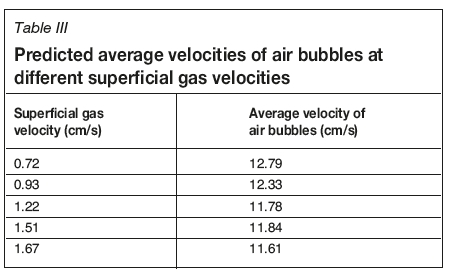
Table III shows the volume-weighted average velocity of air bubbles obtained from the CFD simulations at different superficial air velocities. For the constant bubble size of 1 mm used in the CFD simulations, the average bubble velocity seems to decrease slightly with increasing superficial gas velocity. This is perhaps due to the increase in average gas holdup (volume fraction) resulting from the increasing superficial gas velocity (López-Saucedo et al., 2011; Nicklin, 1962; Zhou, Egiebor, and Plitt, L. 1993). When bubble volume fraction or gas holdup is increased, the drag force increases hence the bubble velocity decreases.

 

 

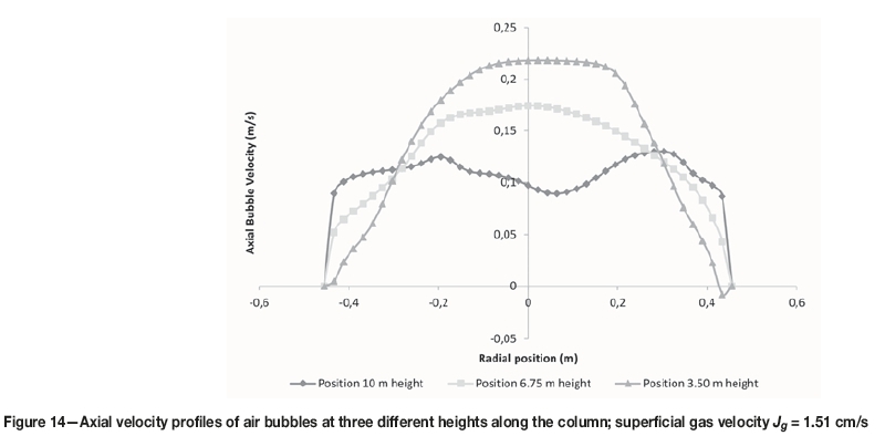
The simulated axial velocity profiles of air bubbles at different heights in the column are shown in Figure 14 for Jg = 1.51 cm/s. It can be seen that the axial bubble velocity decreases with height along the column. Previous research on axial velocity profiles of single bubbles identified similar bubble behaviour along the column height due to the progressive increase in the drag coefficient resulting from surfactant-induced changes at the bubble surfaces (Sam, Gomez, and Finch, 1996). However, since the effects of surfactants on bubble surfaces are not accounted for in the present CFD model, the observed axial variation in bubble velocity in this case must have its origins in some other mechanism, possibly the increase in the drag force resulting from the increase in gas holdup with height along the column. The observed decrease in bubble velocity with height could result in an increase in bubble residence time and this may cause a further increase in the axial gas holdup profile. Figure 14 also shows a change in the shape of the axial bubble velocity profile from a parabolic shape at the bottom and in the middle to a more uniform profile at the top of the column where the flow turbulence is fully developed.

In Figure 15, the axial velocity of bubbles is plotted against height along the column axis. The velocity profile obtained shows three stages, similar to the three-stage profile described by Sam, Gomez, and Finch (1996) for single bubbles rising in a 4 m water column in the presence of frother. In the initial stage, the bubble velocity increases rapidly (acceleration stage), reaching a maximum velocity of 23.2 cm/s at height of approximately 2.7 m in the column. This value compares favourably with the maximum velocity of 25.0±0.4 cm/s reported by Sam, Gomez, and Finch (1996) for bubbles of 0.9 mm diameter. In the second stage (deceleration stage), the bubble velocity decreases until at a height of approximately 8.5 m. After that, the bubble velocity appears to fluctuate around an average of about 11.5 cm/s (constant velocity or terminal velocity stage). This value can be compared to the terminal velocities of between 11.0 and 12.0 cm/s observed by Sam, Gomez, and Finch (1996) for similar a bubble size (0.9 mm diameter).

 

 

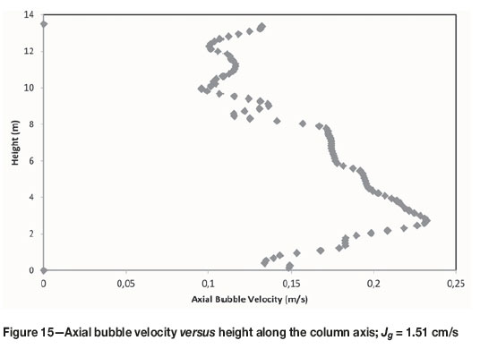
An interesting observation here is that in spite of the fact that this CFD model does not account for the effects of frother, the results in Figure 15 are similar to the three-stage profile described by Sam, Gomez, and Finch (1996) for bubbles rising in water in the presence of frother, where the decreasing velocity in stage 2 was attributed to progressive adsorption of surfactant molecules as the bubble rises. On the other hand, Ishii and Mishima (1984) have shown that the drag coefficient increases with increasing volume fraction of particles (or bubbles) in the viscous and distorted particles regime. The deceleration of bubbles observed in the CFD results could therefore be related to the increase in gas holdup along the column axis due to increases in the drag force.

Comparison of average and axial gas holdup predicted using different drag coefficients

Simulations were also performed to compare the gas holdup prediction when different drag coefficient formulations were used. In this regard, CFD simulations were carried out with three drag models, the universal drag, Schiller and Naumann, and the Morsi and Alexander models. The parity plot comparing the average gas holdup prediction for the different drag coefficients is shown in Figure 16. It can be seen that there is no significant difference between the results obtained with the three drag coefficients.

The average gas holdup results obtained with the three drag coefficients are further compared against experimental data in Table IV in terms of the mean absolute relative error (MARE) between the CFD predictions and the corresponding experimental measurements calculated as follows:

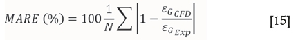
With MARE equal to 6.2%, the universal drag coefficient performs better compared to the Schiller-Naumann (MARE = 7.9%) and Morsi-Alexander (MARE = 10.8%) coefficients.

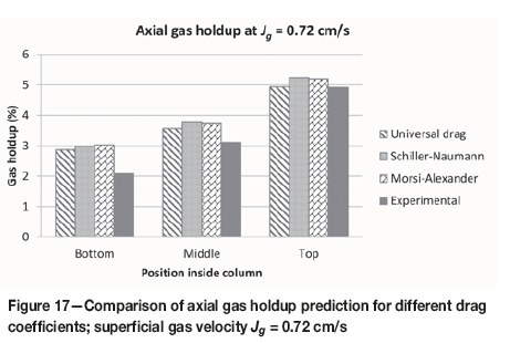
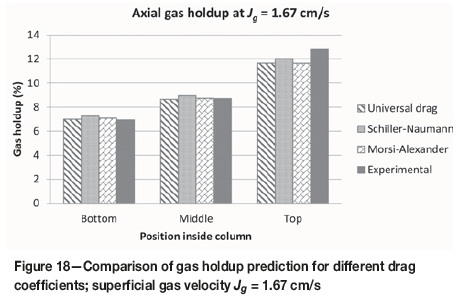
The axial gas holdup predictions using the different drag coefficients are compared with experimental data (Gomez et al., 1991) in Figure 17 and Figure 18. There is again no significant difference between the results obtained with the three drag coefficients. For all three drag models, the gas holdup prediction was very good for the middle part of the column, good for the top part, and over-predicted at low superficial gas velocity J_g= 0.72 cm/s) for the bottom part of the column. The over-prediction of the local gas holdup at the bottom part of the column can be attributed to bubble coalescence, as explained above. The mean absolute relative errors calculated for the different drag coefficients for the axial gas holdup prediction are presented in Tables V-VII. A MARE above 20% was obtained for the gas holdup prediction in the bottom part of the column with all three drag coefficients. On the other hand, the gas holdup in the middle and top parts of the column was predicted with less than 10% relative error.

 

 

 

 

Conclusions

CFD modelling was applied to study the gas holdup and its variation along the collection zone of a pilot flotation column. Both the predicted average gas holdup and the axial (local) gas holdup were in good agreement with the experimental data available in the literature. The generally known gas holdup profile, with the gas holdup values increasing upward in the column and having maximum values in the centre of the column, was also predicted by the CFD simulations.

Three drag models, the universal drag, Schiller-Naumann, and Morsi-Alexander drag coefficients, were compared in order to determine the suitable drag model for average and axial gas holdup prediction in the column. The three drag coefficients all produced good prediction of both the average and local gas holdup. Therefore, any of these three drag coefficients can be used to model flotation column hydrodynamics.

An axial bubble velocity profile was also observed in which the bubble velocity magnitude decreased with height along the column. The reason for this could be the increase in drag coefficient resulting from the axial increase in gas holdup along the column height. However, the decrease in axial bubble velocity along the column height can result in a further increase in the axial gas holdup variations compared to the effect of the hydrostatic pressure only. The axial variation in gas holdup could therefore be explained as having its origins in two interrelated processes; the hydrostatic expansion of air bubbles and the development of a bubble velocity profile in which the axial velocity of bubbles decreases with height along the column.

 

Acknowledgements

The authors would like to thank the Nuffic Heart Project, the Copperbelt University, and the Process Engineering Department of Stellenbosch University for providing the funding and facilities which made this research possible. Computations were performed using the University of Stellenbosch's Rhasatsha High Performance Computing (HPC) cluster.

 

Nomenclature

F_D Drag force per unit volume, N/m3

u' Velocity fluctuation, m/s

U Reynolds-averaged velocity, m/s

g Gravitational acceleration, 9.81 m/s²

Ac Column cross-sectional area, m²

C_D Drag coefficient, dimensionless

dß Bubble diameter, mm

Jg Superficial gas velocity, cm/s

k Turbulence kinetic energy, m2/s2

P Pressure, Pa

R Universal gas constant

Re Reynolds number, dimensionless

S_q Mass source term for phase q, kg/m³-s

T Temperature

V Volume, m3

ΔH Separation distance for gas holdup measurement

ΔΡ Pressure difference

Greek letters

T Viscous stress tensor, Pa

eg Air volume fraction or gas holdup

ak Prandtl number for turbulence kinetic energy, dimensionless

σ_εPrandtl number for turbulence energy dissipation rate, dimensionless

ε Volume fraction

_e Turbulence dissipation rate, m2/s3

μ Viscosity, kg/m-s

μ_t Turbulent viscosity, kg/m-s

ρ Density, kg/m³

Subscripts

B Bubble

D Drag

G, g Gas

i, j Spatial directions

L Liquid

q Phase

 

References

Bhole, M., Joshi, J., and Ramkrishna, D. 2008. CFD simulation of bubble columns incorporating population balance modeling. Chemical Engineering Science, vol. 63, no. 8.. pp. 2267-2282.         [ Links ]

Chakraborty, D., Guha, M., and Banerjee, P. 2009. CFD simulation on influence of superficial gas velocity, column size, sparger arrangement, and taper angle on hydrodynamics of the column flotation cell. Chemical Engineering Communications, vol. 196, no. 9. pp. 1102-1116.         [ Links ]

Chen, J., Yang, N., Ge, W., and Li, J. 2009. Computational fluid dynamics simulation of regime transition in bubble columns incorporating the dual-bubble-size model. Industrial & Engineering Chemistry Research vol. 48, no. 17. p. 8172-8179.         [ Links ]

Chen, P., Dudukovi , M., and Sanyal, J. 2005. Three dimensional simulation of bubble column flows with bubble coalescence and breakup. AIChE Journal, vol. 51, no. 3. pp. 696-712.         [ Links ]

Chen, P., Sanyal, J., and Dudukovic, M. 2004. CFD modeling of bubble columns flows: Implementation of population balance. Chemical Engineering Science, vol. 59, no. 22. pp. 5201-5207.         [ Links ]

Delnoij. E., Kuipers. J.A.M., and van Swaaij. W.P.M. 1997. Computational fluid dynamics applied to gas-liquid contactors. Chemical Engineering Science, vol. 52, no. 21-22, pp. 3623-3368.         [ Links ]

Deng, H., Mehta, R., and Warren, G. 1996. Numerical modeling of flows in flotation columns. International Journal of Mineral Processing, vol. 48, no. 1. pp, 61-72.         [ Links ]

Devanathan, N., Moslemian, D., and Dudukovic, M. 1990. Flow mapping in bubble columns using CARPT. Chemical Engineering Science, vol. 45, no. 8. pp. 2285-2291.         [ Links ]

Dobby, G., Amelunxen, R., and Finch, J. 1985. Column flotation: Some plant experience and model development. Proceedings of the IFAC Symposium on Automation/or Mineral Development, Brisbane. Norris, A.W., and Rurner, D.R. (eds). Australasian Institute of Mining and Metallurgy, Melbourne. pp. 259-264.         [ Links ]

Finch, J.A. and Dobby, G.S. 1990. Column Flotation. Pergamon Press, Oxford UK.         [ Links ]

Finch, J. and Hardie, C. 1999. An example of innovation from the waste management industry: Deinking flotation cells. Minerals Engineering, vol. 12, no. 5. pp. 467-475.         [ Links ]

Freedman, W. and Davidson, J. 1969. Hold-up and liquid circulation in bubble columns. Transactions of the Institution of Chemical Engineers and the Chemical Engineer, vol. 47, no. 8. pp, T251-T262.         [ Links ]

Gal-Or, B. and Waslo, S. 1968. Hydrodynamics of an ensemble of drops (or bubbles) in the presence or absence of surfactants. Chemical Engineering Science, vol. 23, no. 12. pp. 1431-1446.         [ Links ]

Gomez, C., Uribe-Salas, A., Finch, J., and Huls, B. 1991. Gas holdup measurement in flotation columns using electrical conductivity. Canadian Metallurgical Quarterly, vol. 30, no. 4. pp. 201-205.         [ Links ]

Gomez, C., Uribe-Salas, A., Finch, J., and Huls, B. 1995. Axial gas holdup profiles in the collection zones of flotation columns. Minerals and Metallurgical Processing, vol. 12, no. 1. pp. 16-23.         [ Links ]

Harach, P.L., Redfearn, M.A., and Waites, D.B. 1990 Sparging system for column flotation. US patent 4,911,826. Cominco Ltd.         [ Links ]

Hernandez, H., Gomez, C., and Finch, J. 2003. Gas dispersion and de-inking in a flotation column. Minerals Engineering, vol. 16, no. 8. pp. 739-744.         [ Links ]

Hills, J. 1974. Radial non-uniformity of velocity and voidage in a bubble column. Tranactions of the Institution of Chemical Enginering, vol. 52, no. 1. pp. 1-9.         [ Links ]

Ishii, M. and Mishima, K. 1984. Two-fluid model and hydrodynamic constitutive relations. Nuclear Engineering and Design, vol. 82, no. 2. pp. 107-126.         [ Links ]

Koh, P. and Schwarz, M. 2009. CFD models of microcel and Jameson flotation cells. Proceedings of the Seventh International Conference on CFD in the Minerals and Process Industries, CSIRO, Melbourne, Australia. CSIRO.         [ Links ]

Koh, P., Schwarz, M., Zhu, Y., Bourke, P., Peaker, R., and Franzidis, J. 2003.: Development of CFD models of mineral flotation cells. Proceedings of the Third International Conference on Computational Fluid Dynamics in the Minerals and Process Industries, Melbourne, Australia. Witt, P.J. and Schwarz, M.P. (eds). CSIRO, Australia. pp. 171-175.         [ Links ]

Kolev, N.I. 2005. Multiphase Flow Dynamics. Vol. 2 Thermal and Mechanical Interactions. 2nd edn. Springer, Berlin.         [ Links ]

Leichtle, G.F. 1998. Analysis of bubble generating devices in a deinking column. MEng thesis, McGill university.         [ Links ]

López-Saucedo, F., Uribe-Salas, A., Pérez-Garibay, R., Magallanes-HernAndez L, and Lara-Valenzuela C. 2011. Modelling of bubble size in industrial flotation columns. Canadian Metallurgical Quarterly, vol. 50, no. 2. pp. 95-101.         [ Links ]

López-Saucedo, F., Uribe-Salas, A., Pérez-Garibay, R., and Magallanes-HernAndez, L. 2012. Gas dispersion in column flotation and its effect on recovery and grade. Canadian Metallurgical Quarterly, vol. 51, no. 2. pp. 11-17.         [ Links ]

Massinaei, M., Kolahdoozan, M., Noaparast M., Oliazadeh, M., Yianatos, J., Shamsadini, R., and Yarahmadid, M. 2009. Hydrodynamic and kinetic characterization of industrial columns in rougher circuit. Minerals Engineering, vol. 22, no. 4. pp. 357-365.         [ Links ]

Michèle. V. and Hempel, D.C. 2002. Liquid flow and phase holdup-measurement and CFD modeling for two-and three-phase bubble columns. Chemical Engineering Science, vol. 57, no. 11. pp. 1899-1908.         [ Links ]

Morsi, S. and Alexander, 1972. An investigation of particle trajectories in two-phase flow systems. Journal of Fluid Mechanics, vol. 55, no. 2. pp. 193-208.         [ Links ]

Nicklin, D. 1962. Two-phase bubble flow. Chemical Engineering Science, vol. 17, no. 9. pp. 693-702.         [ Links ]

Paleari, F., Xu, M., and Finch, J. 1994. Radial gas holdup profiles: The influence of sparger systems. Minerals and Metallurgical Processing, vol. 11, no. 2. pp. 111-117.         [ Links ]

Pfleger, D. and Becker, S. 2001. Modelling and simulation of the dynamic flow behaviour in a bubble column. Chemical Engineering Science, vol. 56, no. 4. pp. 1737-47.         [ Links ]

Pfleger, D., Gomes S., Gilbert, N., and Wagner, H. 1999. Hydrodynamic simulations of laboratory scale bubble columns fundamental studies of the Eulerian-Eulerian modelling approach. Chemical Engineering Science, vol. 54, no. 21. pp. 5091-5099.         [ Links ]

Prince, M.J. and Blanch, H.W. 1990. Bubble coalescence and break up in air sparged bubble columns. AIChE Journal, vol. 36, no. 10. pp. 1485-1499.         [ Links ]

Sam, A., Gomez, C., and Finch, J. 1996. Axial velocity profiles of single bubbles in water/frother solutions. International Journal of Mineral Processing, vol. 47, no. 3. pp. 177-196.         [ Links ]

Schallenberg, J., ENß J.H., and Hempel, D.C. 2005. The important role of local dispersed phase hold-ups for the calculation of three-phase bubble columns. Chemical Engineering Science, vol. 60, no. 22. pp. 6027-6033.         [ Links ]

Schiller, L. and Naumann, A. 1935. A drag coefficient correlation. Vdi Zeitung. vol. 77. pp. 318-20.         [ Links ]

Shih, T., Liou, W.W., Shabbir, A., Yang, Z., and Zhu, J. 1995. A new k-g eddy viscosity model for high Reynolds number turbulent flows. Computers & Fluids, vol. 24, no. 3. pp. 227-238.         [ Links ]

Tavera, F., Escudero, R., and Finch, J. 2001. Gas holdup in flotation columns: Laboratory measurements. International Journal of Mineral Processing, vol. 61, no. 1. pp. 23-40.         [ Links ]

Xu, M., Finch, J., and Huls, B. 1992. Measurement of radial gas holdup profiles in a flotation column. International Journal of Mineral Processing, vol. 36, no. 3. pp. 229-244.         [ Links ]

Yianatos, J., Bergh, L., DurAn, O., Diaz, F., and Heresi, N. 1994. Measurement of residence time distribution of the gas phase in flotation columns. Minerals Engineering, vol. 7, no. 2. pp. 333-344.         [ Links ]

Yianatos, J., Bergh, L., Sepulveda, C., and Núnez, R. 1995. Measurement of axial pressure profiles in large-size industrial flotation columns. Minerals Engineering, vol. 8, no. 1. pp. 101-109.         [ Links ]

Zhou, Z, Egiebor, N., and Plitt, L. 1993. Frother effects on bubble motion in a swarm. Canadian Metallurgical Quarterly, vol. 32, no. 2. pp. 89-96.         [ Links ]

Zhou, Z. and Egiebor, N. 1993. Prediction of axial gas holdup profiles in flotation columns. Minerals Engineering. vol. 6, no. 3. pp. 307-312.         [ Links ]

Zhou, Z., Egiebor, N., and Plitt, L. 1993. Frother effects on bubble motion in a swarm. Canadian Metallurgical Quarterly, vol. 32, no. 2. pp. 89-96.         [ Links ] ♦

 

 

Paper received Dec. 2017
Revised paper received Mar. 2018