PAPERS OF GENERAL INTEREST

 

A comparison of indirect lognormal and discrete Gaussian change of support methods for various variogram estimators

 

 

R.V. Dutaut; D. Marcotte

École Polytechnique, Canada

 

 

---

SYNOPSIS

In mineral resource evaluations, geostatistical methods known as global change of support allow prediction of the theoretical histogram and gradetonnage curves prior to interpolations or simulations of grades. Two methods commonly used by professionals to guide the choice of interpolation parameters and assess results are the discrete Gaussian model (DGM) and the indirect lognormal correction (IndLog). These models rely upon an estimate of the dispersion variance of the blocks, which is derived by numerical integration of the variogram model over a discretized block. Due to difficulties in obtaining well-formed traditional experimental variograms (especially in the presence of outliers and limited clustered data), many professionals prefer to use 'normalized' variograms such as correlogram (non-ergodic variogram), pairwise-relative, or variogram of the normal score transform. A series of simulations with different grade distributions and variogram models are used to assess the performances and robustness of the various variogram estimators with respect to the DGM and IndLog global change of support. Our results show that the traditional variogram, the correlogram, and normal score variogram have better performances, compared to pairwise, for both DGM and IndLog. Moreover, DGM provided better results than IndLog for the grade distributions that are not strictly lognormal. These findings provide valuable guides for geostatistics practitioners.

Keywords: geostatistics, variogram type, global change of support, volume-variance.

---

 

 

Introduction

When reporting resource estimates, practitioners are required to follow general standards described in the NI43-101 (CIM guidelines), JORC, or SAMREC codes. One can generally recognize three main parts directly related to the block model:

► Pre-processing: exploratory data analysis (EDA), domaining, capping, compositing, declustering, variography

► Processing: block size, neighbourhood, interpolation types (linear or nonlinear)

► Post-processing: classification, reporting.

Pre-processing aims to simplify and strengthen the processing step. Ideally, domaining, capping. and compositing is aimed at defining a single homogenous population. During the processing phase, a common practice is to use a block size corresponding to the planned selective mining unit (SMU). In most precious metal deposits (gold, notably), the SMU size is frequently smaller than the recommended half data spacing (Journel and Huijbregts 1978), resulting in high estimation variance and either a high degree of smoothing if the regression slope is managed or a high degree of conditional bias if it is not. Most actual resource estimates are made using block sizes between one-quarter to one-sixth of the average data spacing, sometimes even smaller. In addition to the block size, the interpolation choices for the neighbourhood selection and interpolator (e.g. inverse distance (ID) or ordinary kriging) are often based on the Qualified Person's (the QP) experience and some basic validation plots that often do not consider the conditional bias (e.g. trends or SWATHs plots, which are designed to compare two sets of population using a one-dimensional graph).

Based on these findings, Rossi and Parker (1994) proposed to 'tune' the kriging plan so that the distribution of the interpolated estimate has a coefficient of variation close to the theoretical one obtained by a global change of support method (hereafter simply referred as the change of support or COS). Although criticized for the possible introduction of conditional bias (Krige, 1997; Journel and Kyriakidis, 2004), this practice is becoming more common in technical reports. It is mostly applied as a visual check on the grade-tonnage curve or as a Q-Q plot of the grades. This simple technique ensures that the estimated blocks respect the SMU's theoretical global grade-tonnage curves. In its simplest form, practitioners select the interpolant type (OK or ID2-ID3 most of the time), the minimum and maximum number of points (composites) used for the interpolation, and in some cases, the number of points per octant or maximum number of points per drill-hole. Isaaks (2005), Rossi and Deutsch (2013), and Nowak and Leuangthong (2017) stated that during prefeasibility and feasibility studies, resource estimates should seek to respect the global recoverable resources (inferred from COS) rather than providing precise local estimates. Doing so, the estimates are necessarily conditionally biased (David, 1977, chapter 11). Reliable local estimates (free of conditional bias) can be later obtained during production from more abundant grade control data. Journel and Kyriakidis (2004) support the same idea but through the use of simulations.

In order to use the Rossi and Parker (1994) 'tuning method', the practitioner must first select an experimental variogram model and then choose a volume-variance correction algorithm (i.e. a COS model). Even though variogram models and the main COS methods are well-known and have been widely used in the industry for decades, there are only a few publications that have experimentally compared the most widely used methods. Only some authors have compared the available methods from an experimental or practical point of view. Demange et al. (1987) assessed four COS models on skewed data-sets but did not use the IndLog model. Srivastava and Parker (1989) compared the robustness of different variogram types to a lognormal heteroscedastic distribution and concluded that pairwise relative variograms are easier to interpret than traditional variograms; however, they did not measure the impact of the resulting variogram model on estimation or COS. Rossi and Parker (1994) tested global and local COS models, and concluded that the DGM is superior, under the hypothesis that the real ('perfect') variance correction factor was known. Curriero et al. (2002) compared the impact of two variogram types on kriging results; they found that the traditional variogram outperformed the correlogram. Emery (2004) demonstrated some of the limitations of the IndLog, but without direct comparison to the DGM or the impact of variogram estimator. Emery and Ortiz (2005) demonstrated that DGM outperform other COS models for lognormal distribution, but the IndLog model was not assessed. More recently, Chiles (2014) compared two different DGMs and their validity range, but the variogram types were not considered.

We aim to assess the impact of the grade distribution and the choices of the variogram estimator type on the performances of both DGM and IndLog COS models (the latter in two different versions). Three different grade distributions (lognormal, unimodal negatively skewed, and bimodal) and four different variogram estimators (traditional, pairwise relative, correlogram, and normal scores) are compared, using different sampling densities. The goals are to determine for the different distributions considered:

(i) Which variogram estimator leads to estimated models providing more accurate block distribution predictions?

(ii) Which COS provides the best predictions when based on the estimated variogram models from the various variogram estimators?

(iii) How does sampling density affect the performance of variogram estimators and COS models?

We also examine the effect of SMU size on the performance of COS models. We stress that, contrary to most previous papers on the subject, we do not assume the true variogram is known but rather we fit the models to the different experimental variogram estimators. The same fitting criterion and algorithm is used in all cases studied. Hence, the impact of the choice of the fitting method is not considered, and this certainly constitutes a limitation to the study. Also, for simplicity, only 2D cases are considered.

The databases used for comparison are obtained by simulation using the FFT-MA method (Ravalec, Noetinger, and Hu 2000). The methodology section presents briefly the FFT-MA method, the variogram estimators, and the change of support models used. Then for various sampling spacings of simulated data-sets, results of the change of support for different variograms types are examined. Tests on the COS model's sensitivity to block size and variogram range ratios are also studied. Discussions and conclusions follow.

 

Methods

We use a series of simulated data-sets to assess the performance of different variogram estimators for DGM and IndLog. These two COS models are the most widely used in the mining industry. Simulated data-sets enable us to compute the experimental block distributions of the different realizations and allow comparison between the 'true' results and the estimated results predicted by COS with limited sample data. Four main estimators of variograms are generally found within technical reports: traditional, correlogram (non-ergodic), pairwise relative, and normal score. Each of these variograms were computed on both exhaustive and partial data-sets, with the latter used to mimic different densities of exploration drill-holes.

Simulation and sampling method

Simulations to generate the exhaustive data-sets were performed by fast Fourier transformation with moving average (FFT-MA) (Ravalec, Noetinger, and Hu 2000). The mathematical concept behind FFT-MA simulations shows that a random function can be written as a weighted average of white noises where the weighting function used guarantees the reproduction of the covariance model. In FFT-MA, most of the calculations are done in spectral domain (Liang, Marcotte, and Shamsipour 2016), which allows fast generation of a large number of Gaussian simulations. To simulate different distributions, post-simulation transformations were applied: an exponential transformation for lognormal distribution and Gaussian anamorphosis, based on ranking, for bimodal and negatively skewed distributions. Lognormal, bimodal, and negatively skewed distributions cover typical distribution types found in mineral deposits (especially in precious commodities). FFT-MA simulations were performed in 2D using a unit node spacing and a large square field of one thousand units a side. The 2D results could be interpreted as a large bench in an open pit operation, or as a tabular vein-type gold deposit.

To simulate production or definition drill-hole patterns, realizations were virtually sampled over regular grids at 10 and 50 units spacing. The regular grid removes the need to decluster data, although we stress that declustering is an important step that should be performed prior to any mining estimation. The most widely used declustering methods are cell-declustering (Deutsch, 1989), polygonal or voronoi (Chiles and Delfiner, 2012), and kriging weights (Olea, 2007). Moreover, no measurement error was added to the selected data. For interested readers, Journel and Kyriakidis (2004) describe the impacts of sampling error on mining geostatistical methods.

The variogram estimators

There are four variogram estimators usually found in technical reports (the term variogram is used here for experimental semivariogram, and more generally for any tool describing the correlation of the data as a function of the distance):

► The traditional variogram (Matheron, 1963): defined as half the average squared difference between points separated by a distance h.

► The correlogram or non-ergodic variogram (Isaaks and Srivastava 1989) is a standardized variogram type. The standardization is performed using the averages of both the head and the tail and the standard deviations of the pairs. It is considered to be more robust to outliers and heteroscedastic data-sets (Srivastava and Parker, 1989). It is one of the most commonly used variogram estimators in mining applications.

► David (1977) described two forms of relative variogram: the general relative and the pairwise relative. Both are standardized versions of the traditional variogram. In this paper, the pairwise version was used. In the pairwise relative variogram, the standardization is done with the average of the two values for each pair.

► The normal score variogram (Chiles and Delfiner, 2012; Wilde and Deutsch 2005) is identical to traditional variograms except that the data is first transformed to a Gaussian distribution. The Gaussian transformation reduces the impact of outliers on the variogram and facilitates the modelling. The variogram model must then be back-transformed to the original space.

In addition to the nugget effect, it is a common practice in the mining industry to fit one or two variogram structures. Some practitioners may use more, but most resource geologists use two structures, one for short range and the other one for long range, but both oriented in the same direction. The spherical model is a common model used in public reports. Hence, we choose to fit a sum of two spherical variogram models to the experimental variogram of the raw Z-variable, i.e. obtained after transformation of simulated Gaussian values to grade. The fitting was done automatically using a weighted least-squares method, similar to Cressie (1985). Each spherical component was considered anisotropic with known directions of anisotropy. The automatic fitting procedure was applied with no manual control to limit the bias and subjectivity. Although some automatically fitted models ended up far from the true Z-exhaustive variograms, they were kept in all computations to avoid favouring any of the estimators.

Change ofsupport models

Methods of change of support (COS), also known as volume-variance correction or global estimates, seek to derive the global histogram and grade-tonnage curves at SMU size from point distribution (composites). Regrettably, COS are not systematically included in resource estimates in technical reports, although they are required to obtain SMU grade-tonnage curves necessary to guide block simulation/interpolation. There are numerous COS approaches, including affine correction (Journel and Huijbregts, 1978), Gaussian approach (Matheron, 1978), bi-Gaussian approach (Marcotte and David, 1985), mosaic correction (Demange et al., 1987), indirect lognormal (Isaaks and Srivastava, 1989; Emery 2004), lognormal with three parameters (Krige, 1981), discrete Gaussian (Matheron, 1976; Rivoirard, 1994; Emery, 2007) and LU simulation (Davis, 1987). However, the indirect lognormal correction (IndLog) and the discrete Gaussian model (DGM) methods are commonly used by Canadian resource QPs.

The indirect lognormal method is suited for positively skewed distributions (not necessarily lognormal) observed for most precious metal deposits. It assumes the permanence of the lognormal distribution between data at the point support (Z) and SMUs histograms (Z_SMU). The distribution at the SMU size is inferred from the point data by correcting the variance of the population. We have in this model:

where the equality stands in distribution. Two different approaches can be used to determine the coefficients a and b. The first approach is described in Isaaks and Srivastava (1989), hereafter referred to as 'traditional IndLog'. One determines first b:

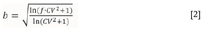
with/the variance correction factor given by:

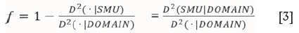
where Z>₂ is the dispersion variance and CV is the coefficient of variation of the point data (Z);/ can be inferred from the variogram model as the ratio of the SMU block variance to the quasi-point variance within the domain. As it is a ratio, it is insensitive to the true sill value (i.e. normalized variograms can be used without re-scaling to population variance).

Parameter a is then chosen to ensure equality of the mean for SMU and point distributions. However, as remarked by Isaaks and Srivastava (1989), multiplication by a*1 does modify the variance of the SMU, thus the correction is not completely consistent.

A better and entirely consistent approach was proposed by Emery (2004), referred in this article as 'Emery IndLog'. First determine b:

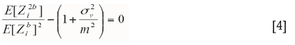
where m = E[Z]. Then, solve the following equation for a:

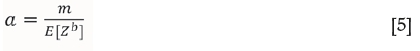
It is easy to verify that these choices ensure the point's mean is preserved and the right SMU variance is recovered. Despite the theoretical superiority of the Emery (2004) approach, most software uses the Isaaks and Srivastava (1989) approach. In our research we assess both methods.

The DGM is slightly more evolved mathematically and interested readers will find more details in Armstrong and Matheron (1986), Rivoirard (1994), Emery (2007), Chiles and Delfiner (2012), or Rossi and Deutsch (2013). The method makes no assumption on the point marginal distribution (Gaussian, lognormal, multimodal, or any other distribution type). Although it is usually presented in textbooks in conjunction with Hermite polynomial expansions to express the transformation from Gaussian to grade variable, this is not a requirement for the method and it can be equally applied using only a graphical transformation. The DGM starts from the Cartier relation:

where Z(x) is the grade of a point randomly selected within block v. Then, assuming that the Gaussian variables Y and Y_vassociated to the grades Z and Z_vfollow jointly a zero mean unit variance bi-Gaussian distribution with correlation r, one can compute (Rivoirard 1994):

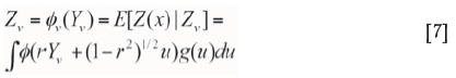
where u is an integration variable, g(u) is the Gaussian density function evaluated at u, and 0(.) is the transformation function from Gaussian Y to grade Zat the point scale. Equation [7] enables a block grade value Zv to be associated with every value of a Af(0,1) distribution (Yv) using simple numerical integration. Note that 0(.) was defined by a simple graphical relation in the present document. In all cases, the only unknown in Equation [7] is the correlation coefficient r. The coefficient r is selected such as to ensure that the transformed Zv variables have the desired SMU variance.

 

Results

Change ofsupport - sensitivity to variogram type.

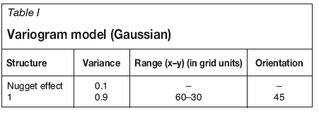
A total of 100 Gaussian simulation realizations are obtained on a grid of 1000 χ 1000 points. The large size of the field (>15 times the correlation range) allows more stable variograms to be obtained; the purpose of this study is not to assess variogram stability as in Srivastava and Parker (1989), but rather the impact of variogram estimators on COS performances. The same variogram is used for all realizations of the Gaussian variable. The variogram is anisotropic with parameters shown in Table I.

 

 

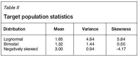
Using Gaussian anamorphosis, three different target distributions for point grade are used: lognormal, bimodal (considered as a single homogeneous bimodal distribution), and negatively skewed. Target distribution statistics are presented in Table II.

 

 

Using all simulated points, the four variogram estimators (traditional, correlogram, pairwise, Nscore) were automatically fitted by assuming a spatial structure composed of a nugget effect and two anisotropic spherical models, both oriented in the same direction. We stress that the fitted model has two structures instead of a single one in the theoretical model as indicated in Table I. This adds flexibility in modelling to account for the effect of the Gaussian anamorphosis on the variogram model. Although a spherical model is used to simulate the Gaussian variable, the variogram of the transformed variable is no more spherical. For each of the four variogram types, DGM and both versions of IndLog change of support were tested using a SMU of the size of 10 χ 10 units. In addition to exhaustive data-sets, each realization was subsampled to imitate regular drill-hole patterns at respectively 1, 10, and 50 units. Then, for each pattern, experimental variograms and COS models were recalculated. This resulted in three patterns χ 4 estimators χ 3 distributions χ 3 COS = 108 possibilities for each cut-off.

Exhaustive data-sets

COS models rely upon an estimate of the dispersion variance to derive distribution at different support size. Using the exhaustive database, Table III compares the mean dispersion variances calculated experimentally from the simulated nodes (real) to the dispersion variances estimated from the different variogram types 10 χ 10 units SMU size. Generally, all variogram types provide close estimates of the true block dispersion variance; although the pairwise variogram systematically underestimates the dispersion variance.

The difference between real (simulated) grades and COS results was then calculated for cut-off grades varying from 0 to 3.3 with a 0.3 increment. Realistic mining cut-offs of 0.3 and 1.5 were selected for plotting (e.g. cut-offs of 0.3 and 1.5 g/t would be reasonable for a gold open pit and a large underground mine respectively). Box plots in Figure 1 present the grade, volume, and conventional profit errors (the conventional profit is defined as P(c) = V(c)(m(c) - c) where c is the considered cut-off and P(c), V(c), and m(c) are respectively the conventional profit, the volume, and the ore grade at that cut-off; it corresponds to the amount of metal left after paying for the costs represented by the cut-off for the three distributions with exhaustive sampling). DGM (blue), traditional IndLog (red), and Emery IndLog (green) are shown. The errors are calculated by subtracting the estimated value from the true value for each realization, so that a positive error corresponds to an underestimation of the parameter. On each box plot, the central mark indicates the median, the box limits correspond to the 25th and 75th percentile, and the whiskers extend to two standard deviations (± 2σ).

For the lognormal distribution, all COS models perform relatively well, while the traditional IndLog shows errors more centred on zero and with a slightly smaller spread. Minimum errors (mean and spread) are obtained with Nscore variograms, whereas the worst results are associated with the pairwise variograms. For distributions that are not strictly lognormal, the DGM appear unbiased; conversely, both IndLog COS models appear biased for most of the statistics considered. Emery IndLog achieves better results than the traditional lognormal correction. Variogram types performed equivalently, except for the pairwise, which returned slightly biased results.

Grade-tonnage curves for the different distributions

Figure 2 presents, as box plots, the results of the simulated COS model for various cut-offs for each distribution at 10 and 50 node spacing using the traditional variogram. These spacings were selected because they could correspond to the drilling spacing for grade control and long-term models in gold projects. As expected, there is a decrease in confidence (larger box plot spread) with the increase of data spacing, for both grade and volume. With increasing cut-off, confidence decreases for grade, while confidence in tonnage is more constant. The error distribution is relatively symmetrical for all COS models. As previously noted, the DGM presents results more robust to the different distributions. For bimodal and negatively skewed distributions, Emery IndLog errors are more centred on the 'real' grade-tonnage curves (no systematic bias) than the traditional IndLog model. This systematic bias of the traditional IndLog is particularly critical in mining applications.

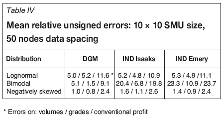
To define an overall measure of performance, the mean relative unsigned errors (MRUE) were calculated over all realizations and all cut-off grades as follows:

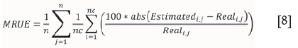
where n is the number of simulations and nc the number of different cut-offs considered.

Table IV presents the MRUE calculated using Equation [8] on the 50-node spacing data-sets and using traditional variogram estimator. DGM outperforms the other models for bimodal distribution and shows a slight advantage for negatively skewed distribution. For the lognormal distribution, all models performed similarly, as expected.

 

 

Change ofsupport - sensitivity to SMU size

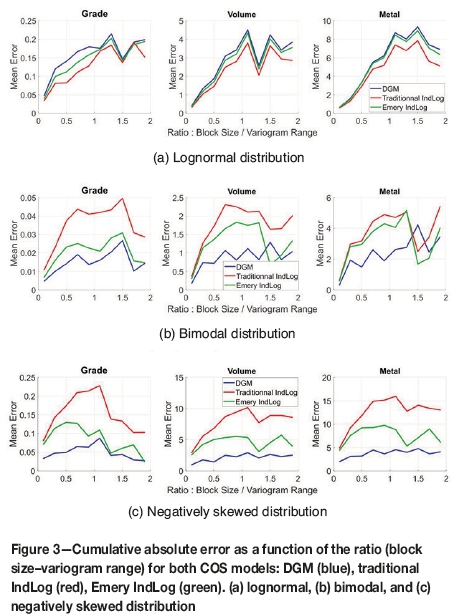
For resource estimates, practitioners must consider the SMU size. This parameter is usually defined as a function of the geological setting, selected mining equipment (shovel-truck size), and other practical resource constraints such as reasonable minimum mining width or software limitations (sub-blocks or partial/percentage blocks). The sensitivity of COS models to block size and variogram range was evaluated for several block size/variogram range ratios. Data-sets were simulated using FFT-MA with a fixed variogram model (isotropic spherical model with a range of 100 units). The exhaustive traditional variograms were computed and automatically fitted. COS models were then compared to simulated SMUs. The exercise was repeated for block sizes ranging from 10 to 200 units, corresponding to ratios 0.1 to 2.

Figure 3 presents the grade and volume mean absolute error (at all cut-offs) for each COS model as a function of the ratio. For lognormal distribution, COS models present relatively similar results, with an error that comprehensively increases with the block size. For bimodal and negatively skewed distribution, the DGM perform the best, followed by Emery IndLog models and then the traditional IndLog. The increase of error with size of support is expected as the true block distribution departs more and more from the point distribution. Also, differences between COS models are stronger for the bimodal and negatively skewed distribution, where DGM outperforms the other COS models for most ratios.

 

 

Discussion

We compared experimentally the performances of two widely used COS models with respect to choice of variogram estimator, type of grade distribution, sampling density, and SMU size. Three different representative distributions were considered, and four different variogram estimators were automatically fitted for a series of sampling patterns. For computational reasons, the tests were run in 2D rather than 3D and a single variogram model was used for the simulated Gaussian variable. Only regular sampling patterns were considered in order to avoid introducing the declustering method as an additional factor to consider.

Keeping in mind the limitations of this experimental study, our results (Figure 1) indicate that the traditional variogram estimator, the correlogram proposed by Isaaks and Srivastava (1989), and normal score variogram provide the best, or close to best, COS results for all the tested distributions. Our results indicate no clear advantage for the correlogram compared to the traditional estimator, which are the two most widely used variograms estimators in technical reports. Pairwise variograms provide biased results when used for COS purposes, a consequence of the underestimation of block dispersion variance (Table III) for this variogram estimator. For lognormal distribution, the normal score estimator returns COS results with the smallest spread. This is probably due to its robustness to outliers.

Figure 2 clearly indicate that the DGM returns more precise and less biased results than IndLog, particularly in its traditional version and when the grade distribution are not lognormal (Figures 2b and 2c). These findings concur with Emery and Ortiz's (2005) conclusions. As demonstrated in Figures 2a and 3a, in the case of a strictly lognormal distribution, all COS models perform equivalently. DGM and Emery IndLog proved more robust than traditional IndLog to the SMU size/variogram range ratio for other distributions (Figures 2, 3a, and 3b).

COS models seek to estimate the in situ grade distribution at the SMU scale, but the precision of the results depends on the data availability. When less data is available, both the histogram and the variogram estimations are less precise, which in turn adversely affects the COS performance. However, DGM proved to be unbiased for all sampling patterns (Figure 2) and all SMU sizes (Figure 3). In our tests, DGM provides grade-tonnage mean relative unsigned errors (MRUE) varying from 1% to 5% for all distribution types, while errors with indirect lognormal methods can be up to 20% for bimodal distribution (Table IV). In the lognormal case for all COS models, MRUE can stretch up to more than 10% at a higher cut-off. These errors represent a best-case scenario, without any domaining, sampling, analytical, or declustering errors. In a real case, practitioners will probably have higher errors during COS associated with an interpolation process. Therefore, it is recommended to use COS curves as guidelines rather than strict constraints for recoverable resource estimates.

During mining operations, the decision to classify a block as 'ore' or 'waste' is based on the estimated grade at the time of mining, not the true unknown block grade. The more information available, the better the classification. This (usually small) information effect can be incorporated within the COS (Roth and Deraisme, 2001) by simply increasing the variance correction factor (or decreasing the degree of selectivity).

Although DGM proved to be more efficient in our tests, it should not be applied blindly. The quality of the results also depends on important and difficult decisions about domaining (Emery and Ortiz, 2005; Romary et al., 2012) and declustering (Deutsch 1989, Rossi and Deutsch 2013). Moreover, the quality of raw data sampling obviously has an impact (Francois-Bongarcon and Gy 2002). Any bias in the point histogram or variogram will adversely affect the performance of the DGM or other COS method (Journel and Kyriakidis. 2004; Pyrcz et al., 2006; Carrasco, 2010). Despite these reservations, DGM should be recommended in preference to IndLog because of its lack of bias and greater robustness to the sampling density, the type of distribution, and the SMU size.

We did not consider the use of conditional simulations in this study. Despite its possible merits, this method is rarely used in technical reports. One reason is that it is much more computationally intensive than DGM or IndLog. Moreover, the variogram model in simulations is for the Gaussian transformed variable rather than the grade variable as in DGM and IndLog. This choice is therefore expected to have more influence with simulations than with DGM and IndLog. It is also complicated by other sensitive decisions regarding the neighbourhood to use for the conditioning.

 

Conclusions

Our study indicates a clear superiority of the discrete Gaussian model compared to the traditional indirect lognormal approach. The improvement proposed by Emery (2004) increases the quality of the indirect lognormal model, but remains less robust than the DGM with respect to distribution types. DGM is unbiased, and robust to sampling density, SMU size, and distribution types. Our study also reveals that traditional, normal score variogram, and correlogram estimators provide comparable estimates of the dispersion variance used for change of support correction. On the contrary, pairwise estimator should be used with caution as it is more sensitive to the grade distribution.

 

References

Armstrong, M. and Matheron, G. 1986. Disjunctive kriging revisited: Part I. Mathematical Geology, vol. 18, no. 8. pp. 711-728.         [ Links ]

Carrasco, P.C. 2010. Nugget effect, artificial or natural?. Journal of the Southern African Institute of Mining and Metallurgy, vol. 110, no. 6. pp. 299-305.         [ Links ]

Chiles, J.P. 2014. Validity range of the discrete Gaussian change-of-support model and its variant. Journal of the Southern African Institute of Mining and Metallurgy, vol. 114, no. 3. pp. 231-235.         [ Links ]

Chiles, J.P. and Delfiner, P. 2012. Geostatistics: Modeling Spatial Uncertainty. Wiley. 734 pp.         [ Links ]

CRESSIE, N. 1985. Fitting variogram models by weighted least squares. Mathematical Geology, vol. 17, no. 5. pp. 563-586.         [ Links ]

Curriero, F.C., Hohn, M.E., Liebhold, A.M., and Lele, S.R. 2002. A statistical evaluation of non-ergodic variogram estimators. Environmental and Ecological Statistics, vol. 9, no. 1. pp. 89-110.         [ Links ]

DAVID, M. 1977. Geostatistical Ore Reserve Estimation. Elsevier. 384 pp.         [ Links ]

Davis, M.W. 1987. Production of conditional simulations via the LU triangular decomposition of the covariance matrix. Mathematical Geology, vol. 19, no. 2. pp. 91-98.         [ Links ]

Démange, C., Lajaunie, C., Lantuejoul, C., and Rivoirard, J. 1987. Global recoverable reserves: testing various changes of support models on uranium data. Geostatistical Case Studies. Quantitative Geology and Geostatistics, vol. 2. Matheron, G. and Armstrong, M. (eds.). Springer, Dordrecht. pp. 187-208.         [ Links ]

Deutsch, C. 1989. DECLUS: a FORTRAN 77 program for determining optimum spatial declustering weights. Computers & Geosciences, vol. 15, no. 3. pp. 325-332.         [ Links ]

Emery, X. 2004. On the consistency of the indirect lognormal correction. Stochastic Environmental Research and Risk Assessment, vol. 18, no. 4. pp. 258-264.         [ Links ]

Emery, X. 2007. On some consistency conditions for geostatistical change-of-support models. Mathematical Geology, vol. 39, no. 2. pp. 205-223.         [ Links ]

Emery, X. and Ortiz, J.M. 2005. Estimation of mineral resources using grade domains: critical analysis and a suggested methodology. Journal of the South African Institute of Mining and Metallurgy, vol. 105, no. 4. pp.247-255.         [ Links ]

Francois-Bongarcon, D. and Gy, P. 2002. The most common error in applying Gy's Formula in the theory of mineral sampling, and the history of the liberation factor. Journal of the South African Institute of Mining and Metallurgy, vol. 102, no. 8. pp. 475-479.         [ Links ]

Isaaks, E. 2005. The kriging oxymoron: a conditionally unbiased and accurate predictor. Proceedings of Geostatistics Banff2004. Leuangthong, O. and Deutsch, C.V. (eds.). Quantitative Geology and Geostatistics, vol 14. Springer, Dordrecht. pp. 363-374.         [ Links ]

Isaaks, E.H. and Srivastava, R.M. 1989. Applied Geostatistics. Oxford University Press. New York. 561 pp.         [ Links ]

Journel, A.G. and Huijbregts, C.J. 1978. Mining Geostatistics. Academic Press. 600 pp.         [ Links ]

Journel, A.G. and Kyriakidis, P.C. 2004. Evaluation of Mineral Reserves: a Simulation Approach. Oxford University Press. 232 pp.         [ Links ]

Krige, D.G. 1981. Lognormal-de Wijsian Geostatistics for Ore Evaluation. South African Institute of Mining and Metallurgy Johannesburg. 51 pp.         [ Links ]

Krige, D.G. 1997. Block kriging and the fallacy of endeavouring to reduce or eliminate smoothing. Proceedings of the 2nd Regional APCOM, Moscow. Wilke, L. and Puchkov, L. (eds.) 4 pp. http://wwww.saimm.co.za/Conferences/DanieKrige/DGK44.pdf        [ Links ]

Liang, M., Marcotte, D., and Shamsipour, P. 2016. Simulation of non-linear coregionalization models by FFTMA. Computers & Geosciences, vol. 89. pp.220-231.         [ Links ]

Matheron, G. 1963. Les principes de la geostatistique. Rapport N-88, Centre de Géostatistique, Ecole des Mines de Paris. 26 pp.         [ Links ]

MATHERON, G. 1976. A simple substitute for conditional expectation: the disjunctive kriging. Advanced Geostatistics in the Mining Industry.         [ Links ]

Guarascio, M., David, M., and Huijbregts, C. (eds.). NATO Advanced Study Institutes Series (Series C - Mathematical and Physical Sciences), vol. 24. Springer, Dordrech. pp. 221-236.         [ Links ]

Matheron, G. 1978. L'estimation globale des réserves récupérables. Course notes C-75, Centre de Géostatistique, Ecole des Mines de Paris. 28 pp.         [ Links ]

Matheron, G. 1984. Isofactorial models and change of support. Geostatisticsfor Natural Resources Characterization. Verly. G., David. M., Journel. A.G., and Marechal, A. (eds.). Springer, Dordrecht. pp. 449-467.         [ Links ]

MARCOTTE, D. and DAVID, M. 1985. The bi-Gaussian approach: a simple method for recovery estimation. Mathematical Geology, vol. 17, no. 6. pp. 625-644.         [ Links ]

Nowak, M. and Leuangthong, O. 2017. Conditional bias in kriging: let's keep it. Gomez-Hernandez, J., Rodrigo-Ilarri, J., Rodrigo-Clavero, M.E., Cassiraga, E., and Vargas-Guzmán, J.A. (eds.). Proceedings of Geostatistics Valencia 2016. Springer International. pp. 303-318.         [ Links ]

Olea, R.A. 2007. Declustering of clustered preferential sampling for histogram and semivariogram inference. Mathematical Geology, vol. 39, no. 5. pp. 453-467.         [ Links ]

Pyrcz, M.J., Gringarten, E., Frykman, P., and Deutsch, C.V. 2006. Representative input parameters for geostatistical simulation. Stochastic Modeling and Geostatistics: Principles, Methods, and Case Studies, volume II. Coburn, T.C., Yarus, J.M., and Chambers, R.L. (eds.). AAPG Computer Applications in Geology 5. pp.123-137.         [ Links ]

Ravalec, M.L., Noetinger, B., and Hu, L.Y. 2000. The FFT moving average (FFT-MA) generator: An efficient numerical method for generating and conditioning Gaussian simulations. Mathematical Geology, vol. 32. pp. 701-723.         [ Links ]

Rivoirard, J. 1994. Introduction to Disjunctive Kriging and Non-Linear Geostatistics. Clarendon Press, Oxford, UK. 192 pp.         [ Links ]

Romary, T., Rivoirard, J., Deraisme, J., Quinones, C., and Freulon, X. 2012. Domaining by clustering multivariate geostatistical data. Proceedings of Geostatistics Oslo 2012. Abrahamsen, P., Hauge, R., and Kolbj0rnsen, O. (eds.). Quantitative Geology and Geostatistics, vol 17. Springer, Dordrecht. pp. 455-466.         [ Links ]

Rossi, M.E. and Deutsch, C.V. 2013. Mineral Resource Estimation. Springer Science & Business Media. 332 pp.         [ Links ]

Rossi, M.E. and Parker, H.M. 1994. Estimating recoverable reserves: Is it hopeless? Geostatistics for the Next Century. Dimitrakopoulos, R. (ed.). Quantitative Geology and Geostatistics, vol 6. Springer, Dordrecht. pp. 259-276.         [ Links ]

Roth, C. and Deraisme, J. 2000. The information effect and estimating recoverable reserves. Proceedings of the Sixth International Geostatistics Congress. Cape Town, South Africa. Kleingeld, W.J. and Krige, D.G. (eds.). Geostatistical Association of Southern Africa. pp. 776-787.         [ Links ]

Srivastava, R.M. and Parker, H.M. 1989. Robust measures of spatial continuity. Geostatistics. Armstrong M. (ed.). Quantitative Geology and Geostatistics, vol. 4. Springer, Dordrecht. pp. 295-308.         [ Links ]

Wilde, B.J. and Deutsch, C.V. 2005. A new approach to calculate a robust variogram for volume variance calculations and kriging. Annual Report, Centre for Computational Geostatistics, Department of Civil & Environmental Engineering, University of Alberta. 8 pp. http://www.ccgalberta.com/ccgresources/report07/2005-308-y-z_variogram.pdf        [ Links ]

 

 

Paper received Dec. 2017
Revised paper received Apr. 2018