PAPERS OF GENERAL INTEREST

 

First-order exchange and spherical diffusion models of heap leaching in PhreeqC

 

 

P.J. van Staden^I; J. Petersen^II

^IMintek, South Africa
^IIChemical Engineering Department, University of Cape Town, South Africa

 

 

---

SYNOPSIS

PhreeqC is an open-source software designed to perform geochemical calculations. It offers a feature for modelling heap leaching according to the most modern 'dual-porosity' visualization, as well as an extensive database of reactions and equilibria. It should represent an attractive option for modelling the chemical heap leaching of oxidized ores since it requires only the entering of the system characteristics and a minimal amount of coding to formulate kinetic expressions and output parameters.
Both first-order exchange and spherical diffusion PhreeqC models are compared to published short-term pulse-test data (over a few days) and model fits to it. The former is simpler and more convenient to use, but the latter yields more realistic results over longer periods of leaching. Comparisons are also made between PhreeqC and HeapSim, the latter having been acclaimed as the most comprehensive heap leaching model to date. The two models were found to yield very similar results. The observed differences are ascribed to subtle differences in the methods of allocation of reagents to competing reactions and in the methods of advancing the liquid phase between time steps.
PhreeqC is slower to execute than HeapSim, but is more rigorous with regard to solution speciation and permits spatial variation of physical and chemical kinetic parameters. The latter feature makes it well suited to the modelling of the effects of segregation and stratification, which have been identified by a number of authors as phenomena that impact on heap leaching performance but which have not yet been systematically studied.

Keywords: heap leaching, modelling, first-order exchange, spherical diffusion.

---

 

 

Introduction

Heap leaching is a means of extracting metal values, typically from low-grade resources as well as from those with a relatively short life of mine within which to recoup the capital investment. It is commonly practised in many parts of the world; locally in southern Africa a growing number of feasibility studies and actual projects have been based on heap leaching, two examples of which are cited by Tassell (2014, 2015). A major attraction of heap leaching, compared to agitated tank leaching or concentrate production, is the savings in capital and operating costs by elimination of the need for fine milling. Furthermore, the relatively simple process chain of mining, stacking, and circulation of leach solution between the ore pile and downstream recovery plant requires a relatively moderate capital investment. The most important compromise that these savings entail is a relatively slow rate of extraction, and hence the ultimate extent of extraction at which a heap can still be operated economically is relatively low. Due to the apparent simplicity of the process, the complex relationship between the various phenomena that govern the metallurgical performance and financial profitability of heap leaching came to be appreciated only some years after its first large-scale adoption and after some project failures. It was then recognized that it is important to accurately estimate heap leaching process and plant design specifications, to speedily diagnose the performance of operating heaps, and to identify the most suitable measures for correcting underperformance. It further became apparent that the ability to do so relies heavily on the adequate identification of the relevant ore characteristics and on a fundamental understanding of the metallurgical, geomechanical, and hydraulic processes underpinning the heap leaching process (Ghorbani, Franzidis, and Petersen , 2016).

 

Generic value of heap leach modelling

The large collection of published heap leach models of various levels of sophistication, as summarized by Dixon (2003), is evidence of the utility of models for the design and understanding of heap leaching. For example, models have been proposed for applications such as the design of heaps (Jansen and Taylor, 2002), for the characterization of observed heap leaching performance (Miller, 2003), and for providing advice on the means for improving heap leaching performance (Dixon and Petersen, 2003). Modelling can add significant value to laboratory test work results by deeper interpretation of the observations and by predicting performance under various scenarios of operating parameters that were not tested experimentally. As a diagnostic tool, modelling can be used to analyse actual heap-leaching data to determine the critical factors affecting performance, for example whether improvements are more likely to be achieved by a narrower dripper spacing or by more aggressive acid addition.

 

Status of heap leach modelling

The theoretical understanding of the underlying phenomena has been improving. The most authoritative model of heap leaching today is the dual-porosity concept whereby the solution inventory of a heap is considered to be mostly immobile. Mass transport of reagents and leached products occurs by diffusion to and from sparsely distributed mobile flow channels (Petersen and Dixon, 2007a). Physical evidence of this mechanism has been provided by the observation of preferential flow channels below drippers (Petersen and Dixon, op. cit.) and by direct observation of areas of higher and lower liquid saturation (Guzman, Scheffel, and Flaherty 2006), and also through PET-scan imaging of a column packed with ore under HL conditions (Petersen, 2016).

 

Value of a PhreeqC model

The task of coding and the associated need for scripting/compiling software can be barriers to the development of a heap leaching model by heap leaching investigators and consultants who are not routinely involved in software development. These constraints can be largely overcome by the availability of the PhreeqC open-source geochemical freeware, which offers dual-porosity column leaching calculations as a built-in feature for which only the parameters need to be provided. Furthermore, PhreeqC has a built-in database of equilibrium and kinetic parameters for a large collection of minerals and soluble species, thereby obviating the need for the user to find that data. The user only needs to expand and modify the built-in database if and as required (Parkhurst and Appelo, 1999), and the built-in features of the software ensure convergence and stability of the solution.

It would not be onerous to construct a heap leach model in PhreeqC that possesses different physical and reaction kinetic properties in different parts of the heap. In custom-coded software, like HeapSim (Petersen and Dixon, 2007a), which appears to be the most systematically developed and tested heap modelling tool to date, this would require re-coding and recompilation. Apart from the generic applications listed above, this capability would make a PhreeqC model also useful for a study of the effects of segregation and stratification in a heap. Segregation/stratification is widely recognized as an inevitable consequence of current stacking practice, as is evident from Kappes (2002), Gross and Gomer (1992), Kerr (1997), Miller (1998), O'Kane, Barbour, and Haug, (1999), Smith (2002), and O'Kane Consultants (n.d.). However, only O'Kane, Barbour, and Haug (1999) and Wu et al. (2007) have published results of studies on the phenomenon, while Miller (1998) refers to related observations made during chloride tracer tests, leaving segregation/stratification as a topic still worthy of further study.

Need for model calibration

To provide confidence in the model outputs, and to be able to place the model results in context relative to results of earlier published models, it is necessary to compare and calibrate the results of the PhreeqC model with results produced by other models for the same input parameters. In particular, it is necessary to compare the PhreeqC model results with those of other dual-porosity models, because this is the most modern heap leach model concept, as mentioned above. Two such comparisons have been made possible by the availability of pulse-test data published by Bouffard and Dixon (2001), and by the availability of the HeapSim software to the authors. A comparison with HeapSim is of particular importance since it is a very comprehensive model, more so than any other model presented in the public domain (Dixon, 2003). Furthermore, case studies have been based on that software, including those by Dixon and Petersen (2003) and Petersen and Dixon (2007b), so that it has become a benchmark.

The built-in data blocks of PhreeqC allow two generic types of dual-porosity models to be constructed, namely a 'first-order exchange' model and a 'diffusional' model. Both of these PhreeqC models are calibrated to the earlier models to optimize the correlations between the results of the various models for a given set of inputs. This renders the PhreeqC modelling results directly comparable with the published results obtained on the earlier models. In the process, similarities and differences, and advantages and disadvantages of the various models can be explored.

 

Background

Terminology

Various authors inevitably use different terminology, which can cause confusion. PhreeqC terminology is used as the standard in this paper. The names of PhreeqC data blocks, such as MIX and TRANSPORT, appear in capitals throughout this text, because that is the form in which they appear in the software and in the user manual by Parkhurst and Appelo (1999). Other important terms to note are:

► The descriptors 'mobile' and 'immobile' in PhreeqC are termed 'flowing' and 'stagnant' by Bouffard and Dixon (2001)

► What is termed in this text the 'first-order exchange' model equates to the 'mixed side-pore diffusion (MSPD)' model of Bouffard and Dixon (2001)

► What is termed in this text the 'diffusional' model equates to the 'profiled side-pore diffusion' (PSDP) model by Bouffard and Dixon (2001), and is similar to that described by the 'Turner structure' underlying the HeapSim model. A difference is that PhreeqCuses a 'tank-in-series' description of flow between finite solution increments compared to the plug-flow approach of HeapSim.

► The spatial increments used for finite difference description of a heap are termed cells in PhreeqC. The term shift refers in PhreeqC to the advance of the solution inventory of a single mobile cell to the next mobile cell below it. These unique PhreeqC terms will be shown in bold throughout the text.

Measures of concentration

The default units in which solution concentrations are specified in PhreeqC are gmole per kg water (i.e., molal concentration). Because heap leaching involves only relatively low-concentration solutions, unit conversions where required for the calculations shown in this text have equated the 1 kg water basis to 1 litre of solution and molal concentrations to molar concentrations, and all solutions were assumed to possess a density of 1 kg/L. A trial calculation in PhreeqC showed that a 10 g/L Cu²⁺(0.157 molar Cu²⁺) solution in 10 g/L H2SO4 medium has a molality of 0.159 mole Cu²⁺per kg water. Therefore if the 0.159 molal Cu2+ result is treated as if it means 0.159 molar Cu2+, the amount of Cu2+ is overestimated by about (0.159/0.157 - 1), or 1.3%.

Geometry

The diffusional versions of the Bouffard and Dixon and PhreeqC models, as well as the HeapSim model, can consider either linear, cylindrical, or spherical geometry for the immobile space in which diffusion occurs. However, Bouffard and Dixon published only the data generated for spherical geometry, against which the calibration described in this text could be performed. Therefore, only spherical diffusion versions of HeapSim and PhreeqC are considered in this text.

 

Formulations of the dual-porosity leaching mechanism

First-order exchange model

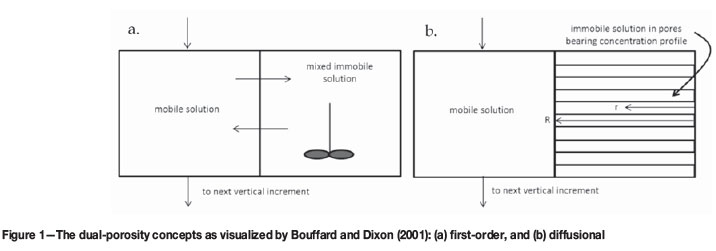
Bouffard and Dixon (2001) proposed two models for the study of the hydrodynamics of solution passing through a packed bed of solids. The first-order exchange visualization shown in Figure 1a divides the mobile pathway into a stack of vertical cells, and associates each mobile cell with a single cell filled with solution that is immobile but of uniform concentration. The governing equation is:

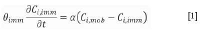
where Ci_¡moband C_i,imm are the solute concentrations (normalized with respect to input and background concentrations) of species i in the aqueous phases contained in the mobile and immobile cells respectively. The term dimm is the volume fraction of the ore bed occupied by immobile solution, α is an exchange coefficient, and t represents time.

Spherical diffusional visualization

In the diffusional model, illustrated in Figure 1b, each mobile cell is associated with pores filled with immobile solution, and dissolved species move to and from the mobile solution by diffusion, driven by concentration profiles in the immobile pores. Bouffard and Dixon (2001) also proposed another version of this model with a non-uniform pore length distribution: in this text only their results obtained with the model with pores of uniform length are considered.

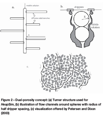
The Turner structure upon which the HeapSim model is based is illustrated in Figure 2a, consisting of a flowing stream of mobile solution from which stagnant diffusional pathways extend into the surrounding ore bed. Figure 2b illustrates how this relates to spherical parcels of ore being irrigated by drippers from above.

 

 

 

 

Both visualizations of leaching with diffusional mass transfer via an immobile zone are mathematically described by Fick's second law of (transient) diffusion. In the absence of chemical reaction and for the case where the side-pores extend into a spherical space of radius R, the transport of chemical species through the stagnant region is, according to the conventions of van Genuchten (1985) and Dixon (2003), described by:

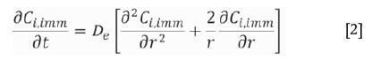
with boundary conditions:

 

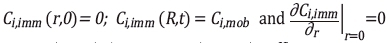
where r is the radial position and D_eis the effective diffusivity of the ore bed matrix. The term De deviates from the free diffusivity D by a factor determined by the tortuosity and restrictivity of the pores containing the immobile solution, which are expected to render D_e< D.

Both the HeapSim and PhreeqC diffusion models utilize Equation [2] to describe diffusion in spherical immobile zones. In the footnote to Table I, comment is provided on the slightly different convention used by Bouffard and Dixon (2001) to formulate their equivalent of Equation [2].

Relationship between the first-order exchange and diffusional models

Although the first-order exchange model of Equation [1] is simpler to use than the diffusional model of Equation [2], the exchange coefficient in Equation [1] does not have clear physical significance. To help overcome this shortcoming, van Genuchten (1985) provided shape factors whereby the exchange coefficient of the first-order exchange model is correlated to the characteristic dimensions of various immobile-zone geometries. According to van Genuchten's relationship for conversion between spherical geometry and the first-order exchange formulation:

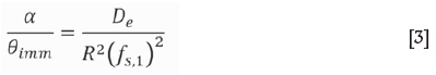
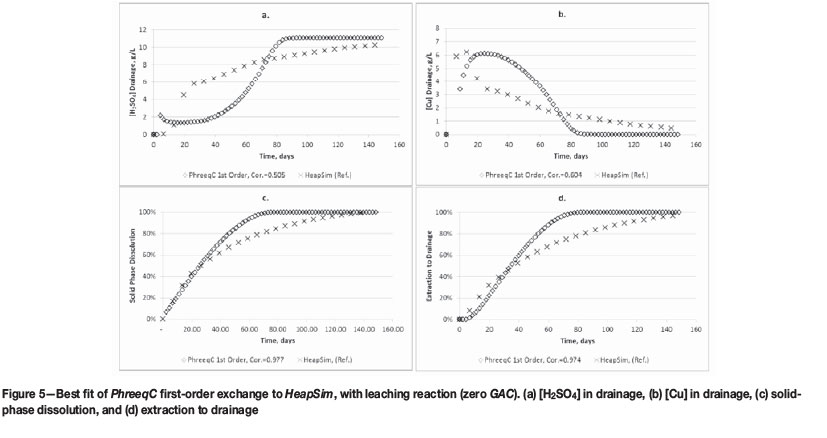
where f_s,1 is a shape factor with value 0.21. However van Genuchten (1985) pointed out that for spherical geometries the conversion did not yield very accurate results, and the same conclusion is drawn in the discussion of the trends observed in Figure 5 below.

 

Figure 5 -Click to enlarge

 

The models in terms of diffusion time

Estimating overall effective in situ values for the tortuosity and restrictivity of diffusional channels in a heap with the aim of obtaining an accurate value of De is quite impractical. Estimating the value of De is further complicated by the fact that any lateral capillary flow will increase the value of De, potentially even rendering it larger than the free diffusivity D, as has been confirmed by Dixon (2003).

Estimating the value of R as about half of dripper spacing on a heap, or half of the diameter of a laboratory column, has been suggested by Dixon and Petersen (2003). That can be visualized as per Figure 2b. However there is not yet sufficient field data available to predict, with any known level of statistical confidence, the likelihood of flow channels below drippers splitting or merging. In fact, the visualization given to dual-porosity hydrodynamics offered by Petersen and Dixon (2003) shows indeed flow channels splitting and merging as per Figure 2c, and this seems to be supported by PET imaging of flow through a column (Petersen, 2016). Furthermore Dixon and Afewu (2011) have calculated the anticipated size of the plume of flowing solution developing below a dripper under the influence of capillary forces. According to their calculations, the advective plume below a dripper occupies a volume typically some hundreds of millimetres in diameter, even under conditions of slow irrigation or within a poorly dispersing ore mass. In such a scenario, the spaces occupied by stationary solution between flow channels must be smaller than half of the dripper spacing, which is also of the order of some hundreds of millimetres.

It is therefore preferred to reformulate Equation [2] into a form that avoids the need to ascribe definitive values to either De or R. This is achieved, analogous to Dixon (2003), by defining the dimensionless radial position (ξ) as

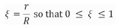
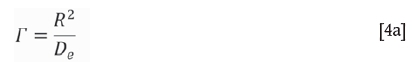
and the 'diffusion time' (Γ), with units of seconds, as:

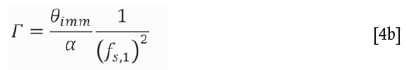
By substitution of the expression for Γ in Equation [4a] into Equation [3], it follows that the diffusion time for the first-order exchange case can also be written as:

For the case of spherical diffusion, Equation [2] can hence be re-written as:

The diffusion time therefore provides a single number for comparison of the hydrodynamics of systems being modelled by the first-order and diffusional models.

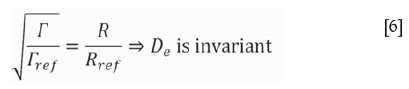
Although the concept of diffusion time now eliminates the direct comparison (in units of length) of the diffusional path lengths of different cases, one diffusional path length ( R) can still be expressed as a fraction of the diffusional path length of a reference case (R_ref) if the two cases are assumed to exhibit the same diffusivity (even though the magnitude of the diffusivity may be unknown) by noting in such a case that:

PhreeqC model set-up

Stability criteria

A feature of the ADVECTION and TRANSPORT data blocks of PhreeqC for simulating percolation through permeable columns is that they are based on the displacement of one mobile cell volume per shift. Accuracy and stability of advection flow calculations in PhreeqC therefore require that the following relationship should always be maintained, according to Parkhurst and Appelo (1999):

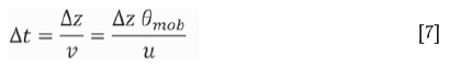
where Δz is the vertical increment length, Δt is the time increment, v is the velocity of flow through the mobile zone, and u is the superficial velocity calculated as the flux per unit area of empty column. This means that Δz and Δt cannot be selected independently by the user: selecting one determines the other.

As will be discussed further below, MIX factors are used in PhreeqC to emulate diffusion in the immobile zone. In doing so, it is a requirement that the amount of solution mixed from any cell to any of its neighbours should always be less than 1/₃(conversely, after mixing each cell should retain at least ¹/3 of its content from the previous time step). This condition can be met by the appropriate selection of Δζ.

Fineness of grid

The PhreeqC calibration was conducted with the number of mobile cells varied from 20 to 75, with very little difference between results and hence only results using 20 and 40 mobile cells are shown. During subsequent optimization, this was further reduced to 10 mobile cells with virtually no noticeable variation in the quality of the results. Because the HeapSim input interface suggests a minimum of four immobile cells per mobile cell, the number of immobile cells in both HeapSim and the PhreeqC diffusional model was kept constant at five per mobile cell for the results presented here. It was verified that PhreeqC diffusional model calculations using four, five, or six immobile cells per mobile cell yielded results that were virtually indistinguishable.

The mobile solution fraction Q_mobdoes not feature in the continuity equation of the diffusional models, as can be seen from Equations [2] and [5], and this applies to both PhreeqC and HeapSim. Therefore parameter Q_mobcan be varied arbitrarily in order to indirectly adjust the time step Δt (as a result of Equation [7]) as large as possible to enhance computational speed, provided it is done within the stability constraint for the MIX factors which are affected by the magnitude of Δt in accordance with Equation [8].

PhreeqC finite difference formulation

The TRANSPORT data block of PhreeqC allows the specification of the number of mobile cells Nz into which the column is divided vertically. Each mobile cell can be associated with either a single immobile cell (to yield a first-order exchange dual-porosity model) or any number N_s> 1 of immobile cells per mobile cell to yield a diffusional dual porosity model.

For the first-order exchange case (N_s = 1) the user needs only to specify the parameters that appear in Table I as inputs. However, to simulate diffusion mass transfer between multiple immobile cells per mobile cell (N_s > 1), the user is required to specify the ratios according to which bordering immobile cells exchange soluble species during each time step. This is a powerful feature since it permits any type of 3D geometry of the immobile cells to be simulated, including the case where immobile cells may be exchanging solutions between different vertical layers. In contrast, HeapSim provides for only linear, cylindrical, or spherical immobile geometries, and diffusion between bordering layers vertically is not allowed.

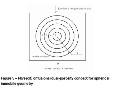
Parkhurst and Appelo (1999) illustrated the equivalence between diffusion mass transfer in the immobile zone and the operation of the MIX data blocks of PhreeqC. Their derivation is briefly repeated here with reference to the concept of a mobile cell containing a spherical immobile zone consisting of five concentric spheres, as illustrated in Figure 3. It is expressed in generic terms of volume (Vj) and contact areas (Akj) so that it remains applicable to any immobile geometry.

Consider the accumulation of a solute in cellj between time t1 and t2 (with t2 = 11 + At, the latter term being the time increment) with cell j being positioned between cells i and k (with i being the stagnant cell to the outside of j, closer to the mobile cell, and cell number k is the cell on the inside towards the centre of cellj). That is to consider only diffusion laterally between cells associated with a single mobile cell, without any exchange vertically between immobile cells, although PhreeqC can accommodate vertical exchange as well. By writing Equation [2] in terms of finite differences for any geometry it follows that:

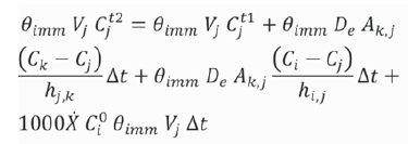
which can be re-arranged after elimination of Ө_imm to yield:

 

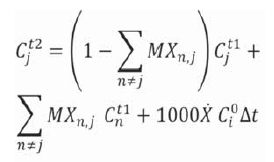
where

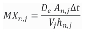
represents the proportion of the content of cell n that is mixed into cell j, where n can be on either side of j, Vj is the volume of cellj, A_n,j is the contact area between cells n and j, and h_n,j is the distance between the mid-points of cells n and j. The mixing factor from cell number n into cell number j is written (for the general case that includes the mobile cell):

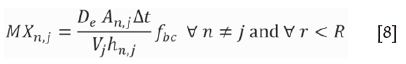
The mixing factor of the central cell j to itself (i.e. the proportion of cell contents of cell j that remains behind after mixing to neighbouring cells), namely MX_jj, is the difference between unity and the sum of the mixing factors to neighbouring cells. Example 13c of the PhreeqC software provides a working model of this type.

The term ƒ_bc is unity for the mixing between all cells inside the spherical immobile zone. For mixing at the boundary between mobile and immobile solution, the diffusional distance h_bc extends from the centre of the outer spherical cell to the boundary wall (opposed to centre-to-centre for diffusion between elements inside the sphere), i.e. h_n,j /2 so that:

for calculating the mixing factor between the outer cell of the sphere and the mobile cell.

It is not simple to eliminate D_e and the terms bearing R (namely A_i,j Vj and h_n,j) from Equation [8] to express it in terms of diffusion time, since the expression needs to provide for the contact area Ai,jon both the inside and outside of spherical shell element j, which prevents terms from being cancelled conveniently. A pragmatic approach for simulating a system with a given diffusion time in PhreeqC or HeapSim would be to adopt any arbitrary value for De (or set it equal to D), and then to calculate the value for R that is required to obtain the desired diffusion time from the expression provided for Γ in Equation [4a].

Kinetic expressions

For the purpose of comparing the PhreeqC and HeapSim simulation results for the cases that included chemical reaction, the kinetic expressions built into HeapSim were used.

The rate of conversion of copper oxide (X_Cuo) is described by:

where K_Cuois the reaction rate constant, C_acidis the molar acid concentration, X is the extent of conversion, and Ø is the exponent on the unreacted fraction. Similarly, the expression used to describe the rate at which acid is consumed by gangue (gangue acid consumption; GAC) is:

with K_gobeing the GAC rate constant.

Mass balance calculations

The HeapSim model performs all calculations, including mass balancing and graphing of the results, and therefore does not require any further calculations from the user. However, PhreeqC provides as outputs essentially the solution compositions, and it is left to the user to calculate from those outputs information such as the percentage extraction and reagent consumption.

PhreeqC requires the solid phase content to be specified in terms of a concentration in the water content of the immobile cells. The initial molal concentration of solid species i in the solution of any immobile cell is specified as:

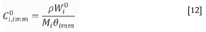
where ρ [kg/m3] is the solid phase bulk density (dry basis), W_i⁰is the mass fraction of species i in the solid phase at time zero, M_iis the molar mass of species i, and Өmm is the volume fraction of immobile solution in the ore bed. The extent of extraction of a solid-phase element i to the drainage solution, X_i,draxn is calculated as the following summation over the number of shifts that have taken place:

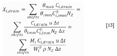
The second and last terms follow by substitution first with Equation [7] and then with Equation [12]. Here, C_itdrain is the concentration in the drainage solution, N_Zis the number of vertical increments, and C_i⁰_,immis defined by Equation [12].

In the case of thefirst-order exchange model, the overall extent of conversion of the solid-phase element i equals the following summation over all immobile cells:

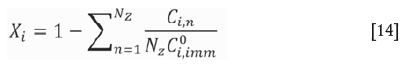
where C_i,n is the concentration of solid species i remaining undissolved in the solution of immobile cell number n, C_i⁰_,immis defined by Equation [12] and Nz is the number of mobile cells (i.e., number of vertical increments which equals the number of immobile cells in the case of the first-order model). This quantity is always slightly higher than the extent of extraction to the drainage solution, by the amount of element i that has been solubilized but has not yet exited the column.

In the case of the spherical diffusion model, the fact that different spherical increments contain different volumes of immobile solution is corrected for by the MIX factors in Equation [8] to calculate the concentration of species in solution correctly. To calculate the extent of extraction from the solid phase, the amount of solid phase allocated to cell number n away from the mobile zone is factored in accordance with spherical geometry, by the factor P_n:

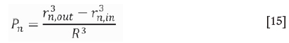
where r_n¡out= R-n.h+h and r_nin= R-n.h, 0 ≤ n ≤ N_s

with Ns being the number of immobile cells associated with each mobile cell ( i.e., the number of concentric spherical increments whereby the immobile phase is represented) and R and r being respectively the radius of the stagnant zone and the distance along the radius.

Therefore, for the spherical diffusion model, the overall average extent of extraction of the solid-phase element i equals the following summation over all immobile cells:

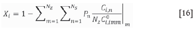
where Ci n is the concentration of element iremaining in the solid phase contained in the solution of immobile cell number n, Ci⁰imm is defined by Equation [12], and Nzis the number of mobile cells (i.e., number of vertical increments).

The total acid consumption (TAC, [kg/t]) is determined from:

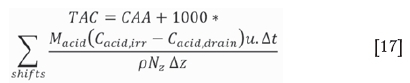
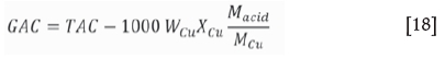
where CAA [kg/t] represents the curing acid addition. For the case where copper is being extracted from an oxide copper mineral such as malachite, one mole of acid is consumed for each mole of copper extracted. Therefore, in that case the acid consumption ascribed to the reaction of gangue constituents, GAC[kg/t], is calculated as the difference between TACand the moles of copper extracted thus:

Integration with Excel

The calculation of MIX factors was automated in Excel, and these were integrated with the PhreeqC data block statements, also in Excel. Charlton and Parkhurst (2011) provided VBA code for an Excel macro whereby PhreeqC statements contained on an Excel sheet can be passed to PhreeqC and the results printed in another Excel sheet, using the PhreeqC Component Object Module (COM). This also facilitates the use of the features of Excel for the mass balance calculations, graphing of results, and statistical analyses. HeapSim offers the same features by operating from an Excel interface, with a predefined set of graphing features as standard

 

Methodology

Short-duration pulse test (no chemical reaction)

Bouffard and Dixon (2001) provided operating parameters as well as the resulting concentration curves (normalized with respect to the background and inlet concentrations) for tracer tests conducted in 1.6 m high columns of ore, using 3.4 M NaNO₃ as inlet pulse against a background of 0.05 M NaNO₃. The pulses had essentially passed through the columns in 4 to 5 days. They optimized the fit of their first-order exchange model to the pulse test data by using the immobile porosity and exchange coefficient as independent variables in a multidimensional optimization routine, minimizing the sum of squared residuals (SSR) between experimental and model data. The diffusional model was fitted using the immobile porosity and diffusional path length ( R) as fitting factors. They also determined the mobile and immobile porosities experimentally as a comparison with the fitted values.

This published experiment was simulated in a PhreeqC first-order exchange model, in a PhreeqC diffusional model, and in HeapSim. Firstly, the published parameters that yielded the best fits between the Bouffard and Dixon model and the experimental data were used as inputs to the PhreeqC and HeapSim models. Secondly, the immobile porosity and exchange coefficient (for the PhreeqC first-order exchange model) and immobile porosity and diffusional path length (for the PhreeqC diffusional model and for HeapSim) were used as independent variables in a two-dimensional Newtonian optimization routine. Optimization was achieved by minimizing the SSR between the model result and experimental pulse test data. One deviation was that the HeapSim model was set up using copper as tracer element instead of sodium, because HeapSim does not provide for sodium as a chemical species; however, the name attached to the chemical species in the model has no bearing on the modelling results: they rely only on the diffusivity being correctly specified.

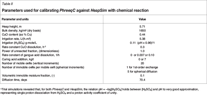
As discussed before, diffusion time is proposed as a comparative characteristic instead of diffusivity and diffusional path length. However, the models still require inputs in terms of the latter two variables in order to effect a required diffusion time, with the understanding that these two variables are not independent but that their ratio contributes towards the diffusion time. Therefore in Table I the diffusivity and diffusional path lengths used in the model calibrations are shown, together with the diffusion time calculated from them.

Long-term leach curve (with chemical reaction)

The batch curves for copper leaching and for GAC were derived from the production and cumulative acid consumption curves of Panel 1 of the Tschudi oxide copper heap leach operation in Namibia, using the methodology proposed by van Staden etal. (2017). This methodology is required where the operational data is generated with irrigation and copper production being initiated while stacking continues. In such a case the production data is generated from ore portions with a range of different leaching ages, so that the rate of copper production versus time does not represent a batch extraction curve. The methodology derives the shape of the batch curve from the copper production data in the form of an exponential decay of the unleached mineral.

The copper extraction and GAC outputs of the HeapSim model were then fitted to the Tschudi batch curves thus determined by manipulation of the input variables to HeapSim. The heap height, bulk density, copper content (represented in this text by the hypothetical mineral CuO), irrigation rate, and acid concentration in the irrigation solution were known from data records. A volumetric immobile solution fraction of 0.1 (equivalent to 0.06 t moisture per ton ore) was assumed from experience. This left (i) the rate constant for copper extraction, (ii) the power of the unconverted copper fraction, (iii) rate constant for GAC, and (iv) diffusional path length (as the means of manipulating diffusion time) as variables to be manipulated to minimize the SSR between model results and the plant leach curve. Firstly, a near-optimal fit of all four variables was simultaneously obtained by trial-and-error, guided by the observations that (a) changes to the GAC rate constant affect the copper leaching and acid consumption curves in opposite ways, (b) changes to the power of the unconverted fraction affect both the duration of the initial linear rate of copper leaching and copper leach rate, without affecting the GAC, and (c) changes to the diffusional path length affect the rate of copper extraction and GAC in similar ways. Finally, the diffusional path length (or diffusion time) was further optimized by a one-dimensional search over a range that included the minimum SSR, keeping the near-optimized values of the other variables fixed.

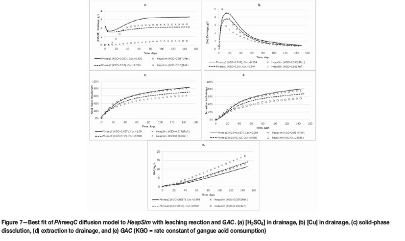
The HeapSim leach curve thus fitted appears in Figure 7 as the data-set labelled 'HeapSim (KGO=0.037)' and served as the reference curve against which both first-order exchange and diffusional versions of the PhreeqC model were calibrated. Arbitrarily selected variations were applied to the GAC rate constant and to the curing acid addition to expand the range of input parameters used for calibration. The diffusional path length (or diffusion time) was used as the sole independent variable manipulated to optimize the data fits between the PhreeqC models and the HeapSim reference curve, using zero GAC and zero curing acid addition. Subsequent comparisons between the models with GAC and with curing acid were performed using the optimized diffusional path length (or diffusion time) with no further parameter fitting.

Correlation coefficients

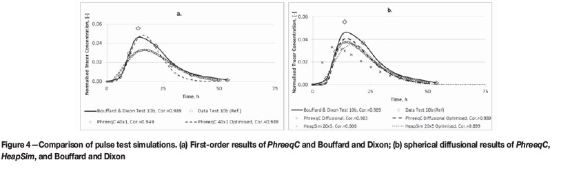
The value of the Pearson's correlation coefficient (which is calculated by the Correl function of Excel), is indicated in the legends of the graphs appearing in this text with the prefix 'Cor.=', to indicate the goodness of fit between data-sets. The reference data set is indicated by 'Ref.' For example, in Figure 4a the experimental data labelled 'Data Test 10b (Ref.)' serves as the reference. The correlation coefficient between the data generated by the first-order exchange version of the PhreeqC model with 40 vertical increments (i.e. with 40x1 vertical by lateral spatial segmentation) and the experimental data is 0.949. This is indicated in the legend of Figure 4a for the results of that PhreeqC model version as 'PhreeqC 40x1 Cor.=0.949'. The experimental data is indicated by diamond markers while the PhreeqC 40x1 calculations appear as circular markers on the same graph, illustrating the fit visually.

 

Results and discussion

Hydrodynamic responses during pulse test simulations

The data published by Bouffard and Dixon (2001) appears in Table I, together with the parameters used and results obtained when their pulse test experiment was emulated in PhreeqC and in HeapSim. The response curves, showing normalized drainage concentration versus time, appear in Figure 4, from which it can be seen that the curves produced by the PhreeqC diffusion model and by HeapSim (Figure 4b) were generally more closely spaced than the PhreeqC first-order exchange results (Figure 4a). None of the three models considered here reproduced the top of the peak observed in the response curve; that was achieved only by a model used by Bouffard and Dixon, which utilized a diffusional path length distribution (as opposed to a single uniform length). That is a feature that has not been included in the PhreeqC models presented here and it is not provided for in HeapSim. Hence no comparison of models with that feature is possible and the results from the Bouffard and Dixon model with the path length distribution are therefore not presented or discussed here.

From Table I it can be seen that the diffusional path lengths (and diffusion times) that yielded the best fits were somewhat lower than those reported by Bouffard and Dixon for both the PhreeqC and HeapSim models, with the HeapSim path length and diffusion time being the shortest. A little more information about the formulation of the model by Bouffard and Dixon, which was coded in MS Fortran Visual Workbench, is provided in the footnote to Table I.

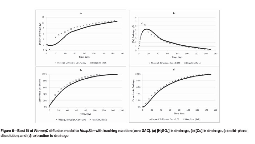
PhreeqC models with leaching reaction, zero GAC

The PhreeqC first-order exchange model was compared with HeapSim for the simulation of the Tschudi heap leach data, using the parameters that appear in Table II and zero GAC. From the graphs and correlation coefficients appearing in Figure 5, the fits can be seen to be quite crude. The inclusion of GAC and curing acid addition in the first-order exchange simulations yielded similar fits and is not reproduced here.

The PhreeqC diffusional model reproduced the trends calculated by HeapSim much better than the PhreeqC first-order exchange model, as evidenced by Figure 6. Both diffusional and first-order exchange versions of PhreeqC attempt to emulate the effect of diffusion from a mobile cell into a lateral channel filled with immobile solution. The first-order exchange model attempts to achieve this in a simplified manner, using a mass transfer coefficient between each mobile cell and its single accompanying immobile cell. During short-lived scenarios of the type appearing in Figure 4, the concentrations between mobile and immobile cells remain sufficiently different to effect significant flow between the mobile and immobile cells. This renders the model behaviour sufficiently sensitive to the value of the mass transfer coefficient to allow short-term pulse data to be fitted by appropriate tuning of the mass transfer coefficient. However, over longer-term simulations of the type appearing in Figures 5 to 8, the concentrations in a mobile cell and the single accompanying immobile cell of the first-order exchange model equalize more readily. It then becomes impossible to accurately emulate the lateral plug-flow of HeapSim (or the lateral tanks-in-series flow of the PhreeqC diffusional model) by tuning of the mass transfer coefficient of the first-order exchange version of the PhreeqC model.

The optimal correlation between HeapSim and the diffusional version of the PhreeqC model was obtained by using the same diffusion time (which appears in Table II) for PhreeqC and HeapSim. Therefore PhreeqC and HeapSim correlate best over longer-period leaching (150 days in this case) when a common diffusion time is used, as opposed to the short-term pulse test (2 days for the data in Figure 4) where HeapSim indicates a shorter diffusion time than PhreeqC.

It is consistently observed throughout Figures 5 to 8 that the PhreeqC model yields apparently early breakthrough of some acid to the drainage solution, which is not observed in HeapSim. This results essentially from a combination of the pH derived from the solution speciation in PhreeqC and the conversion from pH to the effective acid concentrations reported here.

Spherical diffusion model with leaching reaction and GAC

Two simulations were performed with GAC, one using the GAC rate fitted to the Tschudi production data (of 0.037 h-1) and another with a relatively high rate (0.1 h-1). In this case, there is more deviation evident between the two models than was the case with zero GAC, as shown in Figure 7. It is found that PhreeqC predicts a faster rate of Cu extraction and a slower rate of GAC, and the deviation becomes larger with increasing rate of GAC. The somewhat different responses of the [H₂SO₄] curves in Figure 7 are attributed to the different strategies according to which acid is allocated to the competing copper dissolution and GAC reactions. In HeapSim, acid is attributed during each time step to each reaction in proportion to the prevailing reaction rate. In contrast, PhreeqC performs a number of smaller incremental reaction steps within each time step with all reactions in turn, up to the end of the time step or until either reagent or reactant is exhausted.

The calculation of the rate of GAC according to Equation [11] results in the GAC curve in Figure 7e becoming linear once the drainage acid concentration of Figure 7a approaches a pseudo-steady value around day 50.

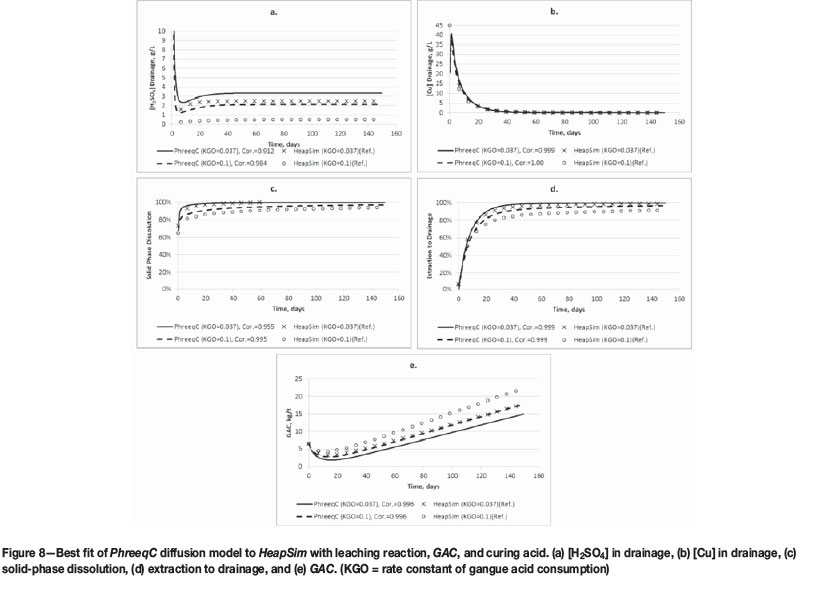
Spherical diffusion model with leaching reaction, GAC and curing acid

When curing acid equivalent to around 45% of the total acid demand over the leaching period is added prior to leaching, the trends coincide much better, as per Figure 8. This is attributed to the more abundant availability of acid to satisfy the requirement of both the CuO and gangue reactions, with less competition for acid.

Due to the differences discussed above in the manner that PhreeqC and HeapSim assign acid to the gangue- and copper-dissolution reactions respectively, the drainage acid concentration is predicted by PhreeqC to drop rapidly from an initial high level, while HeapSim predicts that the acid concentration rises rapidly from a lower value.

Resource optimization

PhreeqC is considerably slower than HeapSim to execute, requiring of the order of ten times the processing time for the spherical diffusion model (e.g., 2.5 minutes vs. 15 seconds to simulate 150 days at a 10-hour time step on a notebook computer with a 2.5 GHz i5 processor). This is primarily attributed to the fact that PhreeqC solves solution speciation calculations during each iteration of each cell, while HeapSim (being custom-coded for a single known application) more pragmatically employs molecular species without considering all possible dissociation reactions.

It is therefore important to optimize the selection of the spatial grid and time interval to achieve rigorous results within the minimum possible processing time. For HeapSim, a minimum of four radial increments, a minimum of eight vertical increments, and a time step of no more than 24 hours are recommended (the time step might need to be shorter if very fast kinetics are involved); these were adopted as a first indication for the minimum standard for PhreeqC.

The PhreeqC processing time is directly proportional to the number of cells and decreases logarithmically with increasing time step size. Due to the relationship between the time step and mixing factor as per Equation [8], changing the time step (or the vertical increment that will affect the time step as per Equation [7]) will affect the MIX factors.

The optimum combination for PhreeqC has been found to be ten vertical increments and a time step of 10 hours, which yields results very similar to those produced by combinations of finer grids and smaller time steps, while still satisfying the stability criterion for MIXfactors discussed above.

 

Discussion and conclusions

The first-order exchange PhreeqC model reproduced published pulse-test data extending over about two days fairly convincingly; however, its correlation to longer-term leach curves was considerably poorer.

The diffusional PhreeqC model emulated more successfully the HeapSim leach curves that had been fitted to 150 days of data from the Tschudi oxide copper heap leach operation in Namibia. This applied to conditions including and excluding gangue acid consumption and curing acid addition. The differences in results obtained in the case where the leaching and GAC reactions were competing for a limited acid supply is attributed to differences in the manner in which the two models assign reagent (H₂SO₄ in this case) to competing reactions. Differences in the methods of advancing the liquid phase between time steps also contributed to some of the observed differences in calculation results.

The HeapSim results fitted the published data of a shortterm pulse test (over 2 days) best with a relatively short diffusion time, compared to the optimally fitted diffusion time required for the PhreeqC models. However the longer-term leach curves (150 days in this case, which of course represents the more practically meaningful application) were optimally fitted by using equal diffusion times for HeapSim and PhreeqC.

One of the disadvantages of PhreeqC compared to HeapSim is that it is slower to execute. Furthermore, heats of reaction and dilution are not accounted for. Therefore PhreeqC does not perform adiabatic calculations, although it allows manual specification of the temperature and pressure of streams and calculates the new temperatures of mixtures of streams with different temperatures. For many percolation-type problems this does not represent a limitation; in fact, it offers the convenience that heats of formation are not required as inputs. However, for oxidative high-temperature heap bioleaching applications, accounting adiabatically for the strongly exothermic reactions and for the heat and mass transfer between the solution and gaseous phases flowing countercurrently would require extensive additional coding by the PhreeqC user.

Advantages of PhreeqC are that it relies on readily available freeware that includes a considerable database of equilibrium and dissociation constants. It further offers a large number of working examples that are likely to include a good starting point for most applications suited to PhreeqC. Little user coding is required and the model structure can very easily be adapted to different uses, making it ideal for engineers and researchers who are not expert coders of modelling software. For example, the different physical and reaction kinetic properties for different parts of a heap can be specified relatively simply, which would facilitate model studies that cannot be done in HeapSim without laborious re-coding. One such example is the modelling of the effects of segregation and stratification on heap leaching performance, phenomena which are widely acknowledged as being of importance in heap leaching, but that have not been studied much to date.

 

Acknowledgements

This paper is published with the permission of Mintek and the University of Cape Town. The operational data made available by Weatherly's Tschudi heap leach operation in Namibia for the 2016 conference paper is gratefully acknowledged. D.L. Parkhurst of the online PhreeqC Users' Forum was helpful in clarifying aspects of mass balancing around PhreeqC TRANSPORT blocks, although the corresponding author accepts all responsibility for the manner in which it has been interpreted and applied in this text.

The modelling results in this paper were first presented in 2016 at the Hydrometallurgy Conference of the SAIMM: Sustainable Hydrometallurgical Extraction of Metals (van Staden and Petersen, 2016). They are presented here with expanded background information as well as improved formulations of the governing mass transfer equations in terms of the diffusion time as the mass transfer characteristic, instead of the combination of diffusivity and diffusional path length. The graphs in Figures 6 to 8 were re-plotted on the basis of a common diffusion time for HeapSim and PhreeqC, and data for a second gangue acid consumption rate was added to Figure 8.

J. Petersen wishes to acknowledge the South African National Research Foundation (NRF) for support under its Incentive Funding for Rated Researchers programme under fund number IPRR UID 85864. The opinions, findings, and conclusions expressed in this paper are those of the authors and the NRF accepts no liability whatsoever in this regard.

 

References

Bouffard, S.C. and Dixon, D.G. 2001. Investigative study into the hydrodynamics of heap leaching processes. Metallurgical and Material Transactions B, vol. 32B. pp. 763-776.         [ Links ]

Charlton, S.R. and Parkhurst, D.L. 2011. Modules based on the geochemical model PhreeqC for use in scripting and programming languages. Computers & Geosciences, vol. 37, no. 10. pp. 1653-1663.         [ Links ]

Dixon, D.G. 2003. Heap leach modelling - The current state of the art. Hydrometallurgy 2003 - Proceedings of the Fifth International Conference. Vancouver., 24-27 August 2003. Vol. 1. Leaching and Solution Purification. Young, C.A., Alfantazi, A.M., Anderson, C.G., Dreisinger, D., Harris, B., and James, A. (eds.). Wiley. pp. 289-314.         [ Links ]

Dixon, D.G. and Afewu, K.I. 2011. Mathematical modelling of heap leaching under drip irrigation. Proceedings of Percolation Leaching: the Status Globally and in Southern Africa, Misty Hills, Muldersdrift, South Africa. Southern African Institute of Mining and Metallurgy, Johannesburg. pp. 81-96.         [ Links ]

Dixon, D.G. and Petersen, J. 2003. Comprehensive modeling study of chalcocite column and heap bioleaching. Proceedings of Copper 2003 - Cobre 2003. Santiago, Chile, 30 November - 3 December 2003. Copper VI: Hydrometallurgy of Copper (Book 2 Riveros, P.A., Dixon, D.G., Dreisinger, D.B., and Menacho, J. (eds.)). Canadian Institute of Mining, Metallurgy and Petroleum. pp .493-515.         [ Links ]

Ghorbani, Y., Franzidis, J.P., and Petersen, J. 2016. Heap leaching technology - current state, innovations and future directions: a review. Minerals Processing and Extractive Metallurgy Review, vol. 37, no. 2. pp. 73-119.         [ Links ]

Gross, A.E. and Gomer, J.S. 1992. Bacterial-assisted heap leaching of ores. US Patent 5196052A. Nalco Chemical Company.         [ Links ]

Guzman, A., Scheffel, R.E., and Flaherty, S.M. 2006. Geochemical profiling of a sulfide leaching operation: a case study. Proceedings of the SME Annual Meeting2006, St. Louis. Preprint 06-014. Society for Mining, Metallurgy and Exploration, Littleton, CO.         [ Links ]

Jansen, M. and Taylor, A. 2002. A new approach to heap leach modelling and scale-up. Proceedings of ALTA 2002 Copper-7 Conference, Castlemaine, Victoria. Alta Metallurgical Services, Perth, Australia.         [ Links ]

Kappes, D.W. 2002. Precious metals heap leach design and practice. Mineral Processing Plant Design, Practice and Control. Society for Mining, Metallurgy and Exploration, Littleton, CO.         [ Links ]

Kerr, E.M. 1997. Polymeric combinations used as copper and precious metal heap leaching agglomeration aids. US patent 5833937. Nalco Chemical Company.         [ Links ]

Miller, G. 1998. Factors controlling heap leach performance with fine and clayey ores. Proceedings of ALTA 1998. Alta Metallurgical Services, Perth, Australia.         [ Links ]

Miller, G.M. 2003. Analysis of commerical heap leaching data. Proceedings of Copper 2003 - Cobre 2003, Santiago, Chile. Copper VI: Hydrometallurgy of Copper (Book 2). Riveros, P.A., Dixon, D., Dreisinger, D.B., and Menacho, J. (eds.). Canadian Institute of Mining, Metallurgy and Petroleum. pp. 531-545.         [ Links ]

O'Kane Consultants. (Not dated). Heap leaching. http://www.okc-sk.com/mine-closure-planning/heap-leaching/ [accessed 10 March 2015].         [ Links ]

O'Kane, M., Barbour, S.L., and Haug, M.D. 1999. A framework for improving the ability to understand and predict the performance of heap leach piles. Proceedings of Copper 99-Cobre 99 International Conference, Phoenix, AZ, 10-13 October 1999. Vol. 4.- Hydrometallurgy of Copper. Young, S.K., Dreisinger, D.B., Hackl, R.P., and Dixon, D.G. (eds.). The Minerals, Metals, and Materials Society, Warrendale, PA. pp. 409-419.         [ Links ]

Parkhurst, D.L. and Appelo, C.A.J. 1999. User's guide to PhreeqC (Version 2) -A computer program for speciation, batch-reaction, one-dimensional transport, and inverse geochemical calculations. US Geological Survey, Denver, Co.         [ Links ]

Petersen, J. 2016. Heap leaching as a key technology for recovery of values from low-grade ores - a brief overview. Hydrometallurgy, vol. 165. pp. 206-212.         [ Links ]

Petersen, J. and Dixon, D.G. 2003. The dynamics of chalcocite heap bioleaching. Hydrometallurgy 2003. Proceedings of the Fifth International Conference. In Honor of Professor Ian Ritchie. Vol. 1. Leaching and Solution Purification. Young, C.A., Alfantazi, A.M., Anderson, C.G., Dreisinger, D. Harris, B., and James, A. (eds.). Wiley. pp. 351-364.         [ Links ]

Petersen, J. and Dixon, D.G. 2007a. Modeling and optimisation of heap bioleach processes. Biomining. Rawlings, D.E. and Johnson, D.B. (eds.). Springer-Verlag, Berlin/Heidelberg. pp. 153-176.         [ Links ]

Petersen, J. and Dixon, D.G. 2007b. Modelling zinc heap bioleaching. Hydrometallurgy, vol. 85. pp. 127-143.         [ Links ]

Smith, E.M. 2002. Potential problems in copper dump leaching. Mining Magazine, July. pp. 1-10.         [ Links ]

Tassell, A. 2014. Kipoi, a nearly perfect copper mining project. Modern Mining, vol. 10, no. 1. pp. 62-63.         [ Links ]

Tassell, A. 2015. Weatherly gets to grips with Tschudi start-up problems. Modern Mining, May. p. 19.         [ Links ]

Van Genuchten, M.T. 1985. A general approach for modeling solute transport in structured soils. Proceedings of the 17th International Congress: Hydrogeology of Rocks of Low Permeability, Tucson, AZ. International Association of Hydrogeologists. pp. 513-526.         [ Links ]

Van Staden, P.J., Kolesnikov, A.V., and Petersen, J. 2017. Comparative assessment of heap leach production data - 1. A procedure for deriving the batch leach curve. Minerals Engineering, vol. 101C. pp. 47-57.         [ Links ]

Van Staden, P.J. and Petersen, J. 2016. A Phreeq C model of heap leaching. Proceedings of Sustainable Hydrometallurgical Extraction of Metals, Cape Town, 1-3 August 2016. Southen African Institute of Mining and Metalluery, Johannesburg. 12 pp.         [ Links ]

Wu, A., Yin, S., Yang, B., Wang, J., and Qui, G., 2007. Study on preferential flow in dump leaching of low-grade ores. Hydrometallurgy, vol. 87 pp. 124-132.         [ Links ]

 

Nomenclature

Abbreviations

CAA Curing acid addition

CoM Component object Module

Cor. Pearson's correlation coefficient

GAC Gangue acid consumption

TAC Total acid consumption

VBA Visual Basic for Applications

Roman symbols

A_i,j Contact area between cells i and jin the PhreeqC diffusional model

C_i,j Concentration of soluble species i in phase j [gmol/L]; [gmol/kg_solution]

C_i⁰_,j Initial (t = 0) concentration of soluble species i in phase j [ gmol/L]; [gmol/kg_solution]

Cor. Pearson's correlation coefficient

D Free diffusivity of dissolved species in solution [m²/s]

D_e Effective diffusivity through the ore matrix [m²/s]

f_bc Correction factor for the mobile/immobile boundary in the equation for MXi,j

ƒ_s,1Shape factor of van Genuchten relating the first-order exchange coefficient to an equivalent diffusional path length [dimensionless]

h Distance between mid-points of neighbouring cells in the diffusional PhreeqC model [m]

K_i Reaction rate constant of species i [h^-1]

Mi Molar mass of species i

MX_i,j PhreeqC MIX factor from a neighbouring immobile cell number i into the central cell number j.

N_s Number of radial (lateral) increments, number of immobile cells associated with each mobile cell

N_z Number of vertical increments

P_n Geometric correction factor for immobile cell number n away from the mobile zone

r Position along the radius of the immobile zone [m]

R Radial dimension of the immobile zone [m]

t Time [h]

Δt Time increment [s], [h], or [d]

u Superficial solution flow velocity [m3/(m2.h)]

v Velocity of solution flow through the mobile zone [m/h]

V_j Volume of cell j in the diffusional PhreeqC model [m3]

W_i⁰ Mass fraction of species i in the solid phase at t = 0

X_i Extent of conversion of species i [dimensionless]

X_i Rate of conversion of species i, [h^-1]

Δz Vertical increment [m]

Greek symbols

α Exchange coefficient between mobile and immobile cells of the first-order exchange models [s^-1]

Г Diffusion time [s]

θ_mob, θ_immThe volumetric fraction of the ore bed occupied by respectively mobile and immobile solution [dimensionless]

ξ Dimensionless distance along the radius of the immobile zone

ρ Bulk density [kg/m3]

Φ Power of the unreacted fraction [dimensionless]

 

 

Paper received Jun. 2017
Revised paper received Oct. 2017