PAPERS OF GENERAL INTEREST

 

Automatic generation of feasible mining pushbacks for open pit strategic planning

 

 

X. Bai^{I, II}; D. Marcotte^I; M. Gamache^I; D. Gregory^III; A. Lapworth^IV

^IDepartment of Civil, Geological and Mining Engineering, Polytechnique Montréal, Canada
^IIGERAD & Department of Mathematics and Industrial Engineering, Polytechnique Montréal, Canada
^IIIDatamine Software Ltd., Sudbury, Canada
^IVDatamine Software Ltd., Wells, UK

 

 

---

SYNOPSIS

The design of pushbacks in an open pit mine has a significant impact on the mine's profitability. Automatic generation of practical pushbacks is a highly desirable feature, but current automatic solutions fail to sufficiently account for complex geometric requirements of pushbacks, including slopes, phase bench and bottom width, smoothness, and continuity. In this paper, we present a tool to fill this gap. Our proposed algorithm is based on modification of sets of blocks obtained by parametric optimization of the pit using a maximum flow method. A set of geometric operators is developed to modify the sets to present a feasible geometry for mining. The geometric operators are essentially derived from mathematical morphological tools. Case studies show that the proposed method generates practical pushback designs that meet all geometric constraints. The algorithm can be used to create a solution for medium-size pits in minutes. This significantly improves the efficiency of designing pushbacks for open pit mines.

Keywords: pushbacks, geometric constraints, bench width, open pit planning, image processing, mathematical morphology.

---

 

 

Introduction

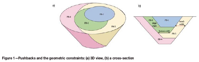
In surface mining, planning over the entire mine life is called long-term planning or strategic mine planning. It involves creating mine designs and schedules on a strategic scale, and provides a financial vision for a project as well as an engineering guidance for short-term production. One of the tasks of strategic planning is to design pushbacks, also referred as cutbacks, periods, or stages (Hustrulid and Kuchta, 1995; Whittle, 2011). Pushbacks (Figure 1) are essentially a series of manageable exploitation phases for an open pit mine. A pushback is ideally composed of a unique, spatially contiguous volume that can be mined with available mining equipment and that meets practical geometric mining constraints. A pushback is typically excavated in a continuous period of one to two years, and the extracted material needs to be able to feed the requirement of processing plants. Sometimes, if mining capacity is available, multiple pushbacks are mined concurrently, to produce sufficient ore to meet production schedules. Practical considerations result in two categories of constraints on pushback design: (i) geometric constraints; space is required for haul road design and machine access, and geotechnically controlled slope angles must be honoured for safety, and (ii) quality and overall size constraints on the content of each pushback to meet production targets, required blends and mill processing capacity etc. Recent literature has primarily focussed on the second category of constraints. Important, but commonly neglected, geometric constraints include minimum mining width, continuity and smoothness. The minimum mining width depends on the mining method and the selected equipment. Smoothness and continuity are critical (Hustrulid and Kuchta, 1995) for facilitating mining operations, specifically by reducing costly movement of equipment and fostering the design of even low-gradient access ramps with the least possible number of turns. Automated pushback design methodologies that implement these constraints are rarely reported in the public domain. This paper seeks to fill this gap.

Many publications on pushback generation emphasize maximization of NPV under resource constraints, with little attention paid to geometric considerations (Consuegra and Dimitrakopoulos, 2010; Goodfellow and Dimitrakopoulos, 2013; Meagher, Dimitrakopoulos, and Vida, 2015). Crucial operational parameters such as mining width, pit smoothness, and continuity have been neglected, resulting in impractical pushbacks. Designs typically include narrow benches and pit bottom, irregular boundaries, and multiple separated components. Post-modification of impractical pushbacks so as to be mineable is a questionable matter. It requires lengthy manual intervention, destroys value, and violates the resource constraints used to obtain the initial design. It is clear that the geometric problem must be dealt with prior to, or simultaneously with, the resources constraints. This is the main aim of this paper.

A few practical pushback generation tools that aimed at creating practical geometries have appeared in the commercial field. GEOVIA Whittle has a Mining Width Module that allows mining width templates to be specified in the X and Y directions and is applied to modify a set of pit shells to fulfil width requirements on benches and at pit bottoms (Whittle, 1998). It can also tolerate benches tapering towards highwalls. NPV Scheduler also includes a pushback generator that modifies nested pits to cater for mining width (Datamine, 2014). BHP Billiton's in-house software 'Blasor' incorporates a tool that can assist manual pushback modification (Stone et al., 2004). More recently, DeepMine software reported a solution that can create the cohesive pushbacks and follows basic operational constraints (Juárez et al., 2014). The tool uses an approximate dynamic programming method for searching the solution space of possible phase configurations. The technical description of these commercial tools is not publicly accessible, and very little detailed information is revealed on the critical functions of controlling pushback geometries.

A few attempts to automatically include geometric constraints are found in the underground mining literature (Bai, Marcotte, and Simon, 2014, 2013a, 2013b; Deraisme, Fouquet, and Fraisse, 1984; Nelis et al., 2016). In particular, Deraisme, Fouquet, and Fraisse (1984) used mathematical morphology operators to produce mineable underground stopes. We exploit this idea in the more challenging context of open pit mining.

In this paper, we focus on the satisfaction of geometric constraints while maintaining a global NPV close to the one obtained using parametric nested pits that do not consider the geometric constraints of minimum width, smoothness, and continuity. We present a new tool to automatically generate pushbacks with all the geometrical constraints fulfilled. The tool is based on a series of new and existing geometric operators that automatically modify an initial parametric pushback to be practical. The geometric operators are based on image processing tools, mainly the mathematical morphological techniques. The tools are embedded in a strategy ensuring that: (i) the resulting NPV remains close to the one obtained with parametric nested pits, and (ii) the ore tonnage available at each period stays within specified bounds.

The paper is structured as follows. We first review the concepts of block model, ultimate pit, and parametric pit. Then, we define the three new geometric constraints (minimum size, smoothness, and continuity) that we want to impose. The notations and the basic mathematical morphological (MM) tools are described. Then, we present step-by-step the new algorithm based on MM to modify a pushback so as to satisfy the new constraints. We then compare the method to the pushbacks based on parametric nested pits that are available in some of the most popular commercial software. We test the algorithm on a simulated deposit and a real copper deposit and discuss its performance. We briefly discuss the computational aspect before concluding.

 

Definitions and notations

In this section, we review the main stages of pushback generation, the notation, and the MM operators used in our approach.

Main stages of pushback generation

The pushback generation involves three main components:

► The resource model

► The ultimate pit (UPit) and

► The generation of pushbacks.

The resource model

The geological resource is usually represented by a 3D block model. Each block has associated values of attributes such as grade, mineral content (valuable mineral or gangue minerals), processing recovery factors, grindability, etc. The block model is generated using exploration sample data and geostatistical modelling to estimate the block variables at unsampled locations (Chiles and Delfiner, 1999). The block model can be either deterministic, which reflects the best estimates, or stochastic, which provides possible alternative scenarios that reflect the uncertain geological and economic conditions (Marcotte and Caron, 2013).

The ultimate pit

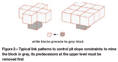
The ultimate pit is the pit that yields the maximum (undiscounted) profit for the given resource model. It comprises a subset of blocks that represent the volume within which the pushbacks should ideally be designed. The pit slope angle requirements are defined by precedence relationships between blocks and can vary at different locations in the mine or along different directions. A simple precedence pattern is shown in Figure 2.

 

 

In operations research, the UPit problem is defined as finding a set of blocks that follows precedence constraints and that yields maximum profit, which is a type of maximum closure problems. The Lerchs-Grossmann (LG) algorithm provides the optimal solution for such a problem (Lerchs and Grossmann, 1965). The equivalent problem can be solved much more efficiently with maximum flow (max-flow) algorithms such as the push-relabel method (Goldberg and Tarjan, 1988) and pseudo-flow method (Chandran and Hochbaum, 2009; Hochbaum, 2008). It is worth noting that the common UPit optimization methods do not consider the minimum mining width of the pit bottom or benches, nor the required smoothness and continuity. Consequently, they usually generate an impractical UPit with areas too narrow to mine or with too many satellite groups of blocks. The UPit, therefore, needs to be modified to ensure feasibility from a mining point of view. The tools developed in this paper can obviously be used for this purpose.

Generation of pushbacks

This step creates spatially connected sets of blocks within the ultimate pit that meet the practical requirements for mining. Common commercial packages use the nested shells method to lead pushbacks generation. Block values can be parameterized by applying revenue factors or cost factors (Whittle, 1988), while running LG or maximum flow on the parameterized models give a series of parametrical pits. As the parameter increases, a series of nested pits can be generated. Each pit only obeys slope constraint and is optimal for the particular economic parameter. Also, inner pits contain higher value per block and are mined before outer pits, therefore optimizing the NPV in a heuristic way. The created pit shells are then selected and modified to form pushbacks that cater for mining width and resources requirements. The great advantage of the nested shell method is that it delivers a range of pit shells for modification very quickly. The efficiency of the method allows large problems to be dealt with.

The procedure for nested pits method can be flexible. A simple way is to use an arbitrary set of revenue parameters and obtain a range of nested pits for further selection and modification, which is adopted by the Whittle tool. A standard optimization-based method is the parametric maximum flow method (Hochbaum and Chen, 2000). Another alternative is to optimize the parameter selection to find pits that best meet the resource constraints. Specifically, the procedure is to iteratively vary the parameter and run max-flow, then check the satisfaction of resource constraints. A satisfied phase is adopted and the procedure moves forward to create following phases. We name this procedure the 'successive max-flow' method. Since our proposed method shares similar workflow, we describe the details of the successive max-flow in Algorithm [11], together with our proposed high-level algorithm.

Geometric constraints for pushbacks: definitions

The slope angle is usually controlled by the precedence relation of blocks. This is a well-documented technique and will not be addressed here. Three other important geometric constraints for pushbacks are: (1) width constraints, (2) smoothness, and (3) continuity.

Width

Sufficient width (typically 100 m) is required on pushback benches (the horizontal sections of one pushback) and pit bottoms, to allow large equipment to work efficiently (Hustrulid and Kuchta, 1995). On the other hand, narrow benches may be mineable with smaller equipment that has a higher cost and lower productivity. Narrow benches should be avoided except in some cases, for example at the edges of pushbacks that are adjacent to a previously mined pit, required to create smooth pit contours. Therefore, the practical requirement of width can be described as two conditions: an area with sufficient target width (TW), or a sub-wide area adjacent to the wide area and to previously mined portions.

Smoothness

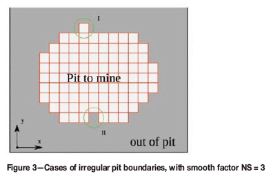
The boundaries of pushbacks are preferably designed to be smooth. Irregular shapes can result in operational difficulties. Irregular shapes can be caused by either small cavities or protuberances at pushback boundaries. The smoothness can be expressed by two conditions: (1) a pit must consist of at least NS consecutively adjacent blocks in both the x and y directions; and (2) if a block is outside the current pushback, it should also have at least NS consecutive adjacent blocks, in both the x and y directions, which are also outside the current pushback. The NS here is the parameter to control the smoothness. The first condition is to eliminate the protuberances of the current pushback, as in case I in Figure 3. The second conditions remove the cavities inside the current pushback, as in case II in Figure 3.

 

 

Continuity

Another requirement of pushbacks is their continuity. The haulage network is a consequence of the pushback design. A pushback comprising multiple disconnected parts would result in separate road access points. This should be avoided because equipment would need to be relocated more frequently within a given period of time, which increases the ramp development and mining costs and the complexity of the operation.

 

Notation

Indexes

i, j, and k Coordinates of a block where k is the level

α, β, and γ Coordinates of a block where γ is the level

t A phase or pushback

Parameters

The number of pushbacks

Tonnage of ore of the phase t

TW The number of blocks to form a wide area for efficient mining operation

AW Auxiliary width parameter to control tolerable sub-wide areas

SE Structural element for morphological operations

SES(w) Structural element of square with width w

NS The parameter to control smoothness

Block elements and sets:

x_i,j,k A block located at (i,j,k)

A block located at

A set of blocks

set of blocks on level k

A set of blocks on level k extracted during phases 1 to t

A set of blocks that have been extracted during phase t, i.e. where and

Duplicated or modified

Duplicated or modified

A set of blocks in a temporarily accepted wide area in the iteration of width controlling algorithm (Algorithm [5])

A set of blocks on level k that are repetitively shifted from modifying pushback and unplanned pushbacks. This is a specific set used in Algorithm [10].

A duplicated or modified

Dilated (enlarged) set

The set of predecessors of blocks , i.e. the blocks that must be extracted if is extracted

The set of successors of blocks , i.e. the blocks that have among their predecessors

The set of successors of blocks in t^th pushback

Basic mathematical morphological tools

From an image processing point of view, a pushback design is a 3D greyscale object where each voxel is valued by the period in which it is mined. A pushback t is a subset of blocks with voxel value t. It can also be represented as a binary image: the voxels in the pushback are indicated by values of unity; others by zeros. Since the width constraints concerns only the horizontal planes, when modifying the width of a pushback, one can focus on the 2D '1-0' image on each level k, where we note Bk is the set of 'unities' .

Mathematical morphological methods are common tools to modify the geometry of images (Serra, 1982) . They are simple and efficient and are very useful for modifying the geometry of objects reflected in the object in an image. The methods are widely applied in image enhancement for the purpose of sharpening, smoothing, edge detection, etc. The characters of the methods are suitable for processing a pushback geometry in our context. The basic morphological tools operate on a binary image, or equivalently a set Bk, with a structural element (SE). The structural element, as a parameter, is a small binary image of a certain shape, like a square, diamond, or other simple shapes. A few basic functions include: (1) dilating, (2) eroding, (3) opening, and (4) closing.

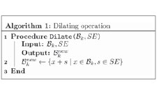
Dilating

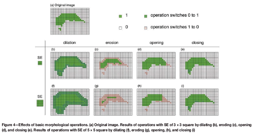
The dilation consists of placing the centre of SE on each element of the set and adding the elements located on SE to the dilated set (see Algorithm [1]). As a result, it returns an extension of the area of '1's in the original image. The dimension and shape of SE defines how the area is enlarged. For example, Figures 4b and 4f show the effect of dilation on the image in Figure 4a respectively with SE of 3 χ 3 square and 5 x 5 square.

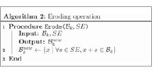
Eroding

The erosion operation (described in Algorithm [2]) has the opposite effect of dilation, i.e. shrinkage of the set . It is also a dual operation of dilation, as eroding a set is equivalent to dilating its complementary set. Similarly, the SE controls the magnitude of erosion. The effect is shown in Figures 4c and 4g.

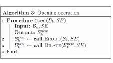
Opening

The opening operation comprises first eroding then dilating (Algorithm [3]). It behaves like matching the pattern of a structural element in the image, and returning only the matched elements. For example, opening with an element of 3 x 3 square on the image of Figure 4a generates the image in Figure 4d, where the parts smaller than 3 χ 3 blocks are removed. Similarly, opening with SE of 5 χ 5 square returns areas with a minimum width of 5 blocks (Figure 4h). It can be seen that the opening is very useful to measure and control the width, as it removes the clusters of blocks that are smaller than the structural element, and keeps the wide areas unaltered.

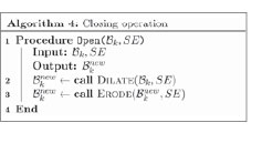
Closing

The closing operation is done by first dilating and then eroding the image (Algorithm [4]). The effect is to join the isolated components that are close to one another, as shown in Figures 4e and 4i.

 

Methodology

Globally, our algorithm defines feasible pushbacks sequentially from the first period to the last. Each pushback is created by modifying the optimal pit obtained by max-flow optimization with a specific price parameter. The parameter value is selected such that the capacity constraints are reached within specified bounds after the enforcement of the geometric constraints. The modification of each pushback proceeds level-by-level, from bottom to top. On each level, the morphological algorithms enforce the constraints of width, smoothness, and continuity, which is the core component of the algorithm. Any modification to a given level implies additional reallocation of blocks on upper or lower levels so as to maintain the slope (or precedence) constraints. Hence, a block added to a given level must come with all its predecessors on upper levels not yet mined in previous pushbacks. Similarly, all the successors of a block removed from a level must also be removed from the current pushback. Once a pushback is obtained, it is considered mined and the max-flow parametric optimization and geometric modifications are rerun on the remaining deposit. This ensures that the new pushback fully accounts for the effect of the geometric constraints applied on the previous pushback.

In next sections, we present the details of algorithms from a low level to high level. We first introduce the 2D geometric operations to control the new geometric constraints. The algorithm to generate a single 3D pushback is then presented. Finally, the main algorithm to create sequentially all pushbacks is discussed.

Geometric operators to control new constraints

We describe in detail the three main new geometric operators used to impose minimal width, smoothness, and continuity.

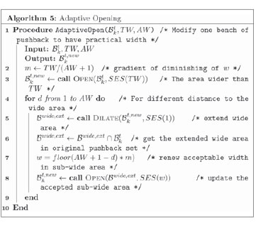
Width operator: adaptive opening

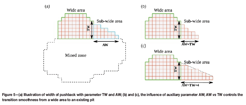
Obtaining the acceptable width of a pushback bench requires two conditions to be controlled: (1) the wide area has a width at least equal to target width (TW), and (2) a small sub-wide area can be mined only if it is adjacent to a wide area and is not too elongated. The first condition is easy to control by the opening operation. For the second condition, the sub-wide area is defined to be acceptable when its shape is roughly a triangle of base length AW, as shown in Figure 5. In this case, the width varies linearly over AW from TW to a single block. The control parameter AW corresponds to the maximum distance a single block can be from the adjacent wide area. Clearly, increasing AW creates a sharper and longer sub-wide zone.

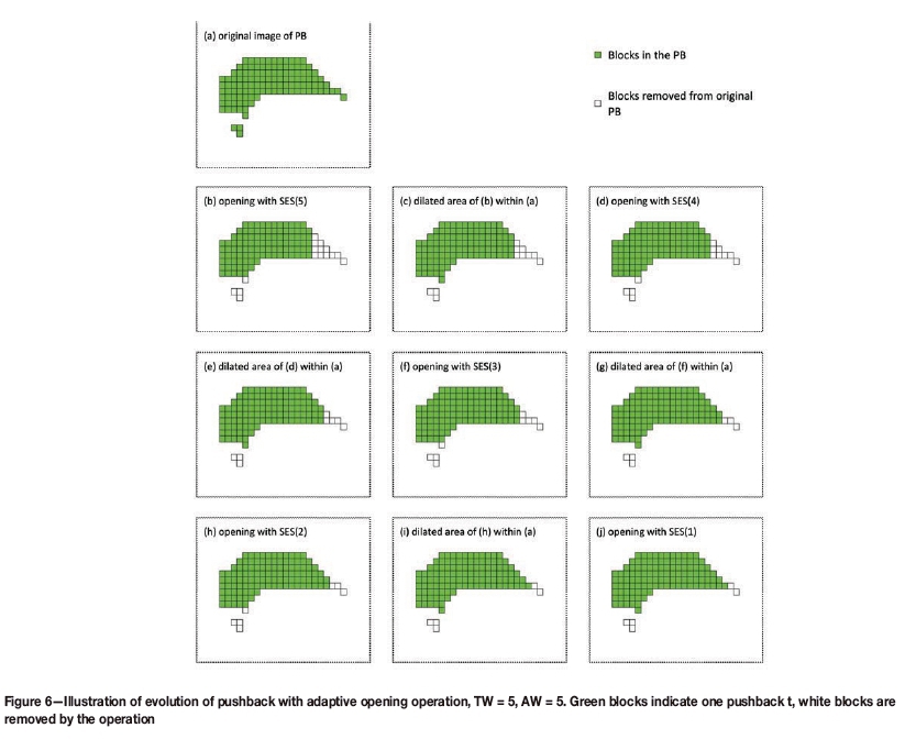
To modify a pushback to have a practical width, we propose a new compound operator based on opening, named 'adaptive opening'. The idea is to first find a set of blocks that satisfy the first width condition, i with minimum width TW. This is done by operating opening on the pushback binary image with a square structural element of size TW (note as SES(w = TW)). This step keeps the blocks that constitute the areas wider than or equal to w, in a set noted as , and removes the others blocks. We then check the abandoned blocks in the original pushback set. If an acceptable sub-wide area adjacent to the wide area can be found, it is added to the wide area . For this, we repeat AW times the following procedure: dilate the area of within the original pushback set, reduce the width requirement w, check if the reduced width can be satisfied on the dilated set, and update the with the newly fulfilled area. The procedure of the adaptive opening is described in Algorithm [5]. A step-by-step evolution of the image during adaptive opening is illustrated in Figure. 6.

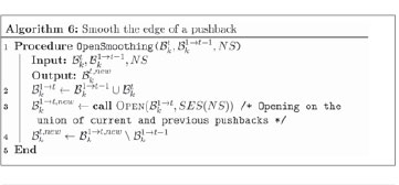
Smoothness operator

To create smooth pushback boundaries, both opening and closing operations are used. Closing can fill the small cave on the edge of pushback, as is shown in Figure 4d. The opening operation cuts the small bumps on the edge of pushback. It should be noted that performing opening on one pushback can also remove the sub-wide transition area created by the adaptive opening. To avoid this side-effect and perform purely smoothing, the opening is operated on the combined set of current and earlier pushbacks, instead of only the current pushback. This procedure is described in Algorithm [6], and is noted as OpenSmoothing. The smoothing factor NS should be smaller than TW, otherwise the smoothing can over-reduce the PB blocks in the area wider than TW. Figure 7 illustrates the effect of OpenSmoothing with factor NS = 3. In Figure 7a, a series of pushbacks is obtained after applying adaptive opening, which is not smooth. In Figure 7b, the yellow blocks represent the union of the current PB and previous PB. We then apply opening with SES(3) on the union of both sets, and obtain Figure 7c. After that, we exclude the previous PB from Figure 7c, and get the new current PB, shown in Figure 7d. These two steps remove the small bumps on the boundary of the current PB, and also avoid removing accepted sub-wide area created during the previous adaptive opening. The result of smoothed pushbacks is displayed in Figure 7e.

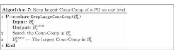
Continuity operator

To control the continuity of a pushback, an algorithm to detect connected components (Conn-Comp) is used (Hopcroft and Tarjan, 1973) . Two cubic blocks can be considered to be connected if they have a shared face. The Conn-Comp identifies the isolated components. The largest connected component is kept; the smaller ones are postponed to later pushbacks. The continuity should be examined not only in 3D, but also in 2D on each level, to avoid an isolated set of blocks on the same level being allocated to the same pushback. The procedure to maintain continuity (KeepLargeConnComp) is described in Algorithm [7].

Synchronizing new geometric operators

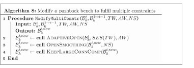
The geometric tools described above control the constraints of width, smoothness, and continuity respectively for one bench of one single pushback. The following sequence of operations is adopted: (1) control the width; (2) smooth (by OpenSmoothing) the pushback edge; (3) keep the largest connected component. The sequence is selected so as to avoid posterior operations altering the previously fulfilled constraints. The three procedures generally remove blocks from the PB. Hence, the 'KeepLargeConnComp' simply removes the disconnected components, and does not change the established width and smoothness. Also, the opening operator in smoothing usually removes the clusters narrower than NS that are not adjacent to previous pushbacks, like the case shown in Figures 7b to 7e. This does not modify the width constraints. The procedure is described in Algorithm [8], and is noted as ModifyMultiConstr.

Multiple pushbacks on a single level

The method to control the geometric constraints for multiple pushbacks is described. Recall that in our algorithm the pushbacks are sequentially generated. When modifying one specific pushback t, the blocks in the ultimate pit can be clustered into three groups: previous pushbacks which include the earlier pushbacks; current pushback ; and future pushback , i.e. the unplanned pushbacks in the ultimate pit. Obviously, the previous pushbacks are already treated and are feasible. For the current PB, modifications should ensure all the geometrical constraints are fulfilled. Also, it should not be ignored that the future PB, the unplanned part, needs also to fulfill the width constraint. Otherwise it can happen that when treating later phases, no valid geometry can be found.

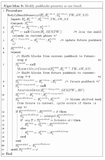
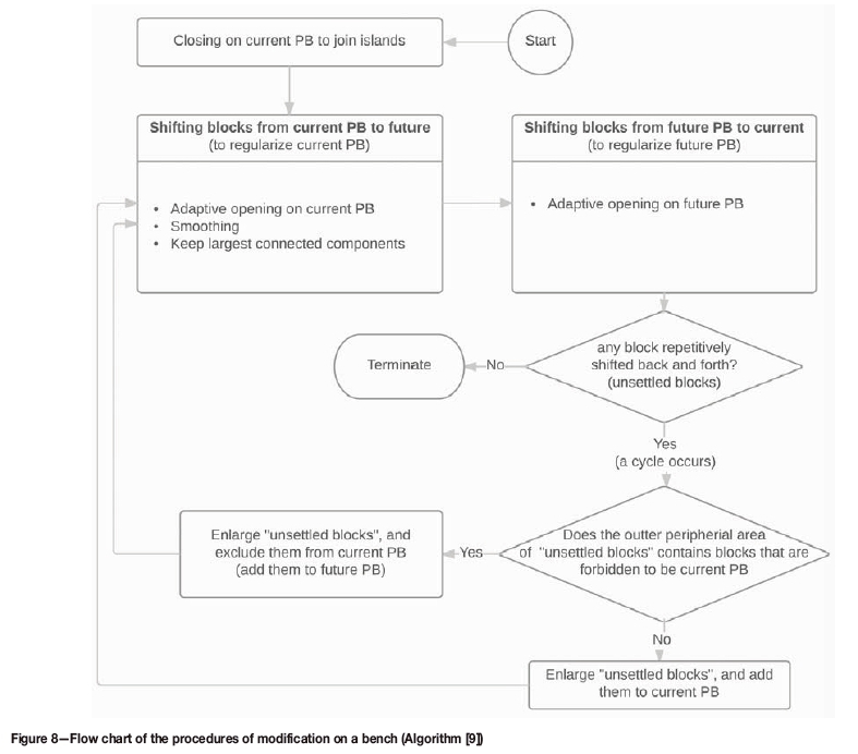
Algorithm [9], noted as 'ModifyBenchGeometry', describes the procedure on a 2D phase bench image. The flow chart is shown in Figure 8. The algorithm includes first a closing operation, in order to join isolated clusters and form a solid area. The closing also has a smoothing effect on the current PB. Then, we apply the geometric functions iteratively on current and future pushbacks, until both of them satisfy all the constraints. For current and future pushbacks, different operations are used. First, the function ModifyMultiConstr (Algorithm [8]) is performed on the current pushback, to make it satisfy the constraints of width, smoothness, and continuity. Then, for future phases, the adaptive opening is operated, because only the width constraint needs to be maintained for the future phase. The iteration essentially shifts blocks repetitively between current and future pushbacks. When operating on current pushbacks, excessive blocks are removed and postponed to future pushbacks, leaving the the current pushback feasible. Similarly, when modifying the future pushback, the removed blocks are moved to constitute the current one. Sometimes, the shifting may not find feasible configuration for both sets of current and future pushbacks, i.e. a cluster of blocks (note as ) is shifted back and forth, and cannot be accepted by either set. This is because the repeated operations change shapes in the same fashion and lack flexibility. In this case, two choices are available: (1) enlarge such cluster and append it to the current pushback, or (2) aggregate neighbouring blocks from the current pushback to enlarge the future pushbacks. The second choice is selected if any of is forbidden from appearing in the current pushback t, otherwise the first choice is applied. The reason a block is banned from pushback t is that some of its predecessors are excluded at upper levels.

Figure 9 illustrates a step-by-step evolution of the pushback bench in Algorithm [9]. Figure 9a shows the original pushbacks, where green blocks stand for the current PB, the white ones for the previous PB, and the grey ones for the future PB. First, we run closing on the current PB, and the isolated blocks are joined (Figure 9b). Next, apply procedure ModifyMultiConstr (Algorithm [8]) on the current PB to make it feasible (see Figure 9c). Then, use adaptive opening on the future PB, to make it wide enough, and move the narrow clusters (grey blocks at left-bottom of Figure 9c) to the current PB. This obtains the result in Figure 9d. After that, repeatedly applying geometrical operations on the current and future PB, obtains Figures 9e and 9f, respectively. It can be seen that a block marked as 'O' is shifted back and forth and cannot be settled. So, we dilate the blocks 'O' inside the union of current and future PBs, then move the dilated block set (block 'O' and '+') to the current PB, and obtain Figure 9g. The procedure ends up with current and future PB both satisfying the geometric constraints.

3D modification of single pushback

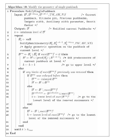
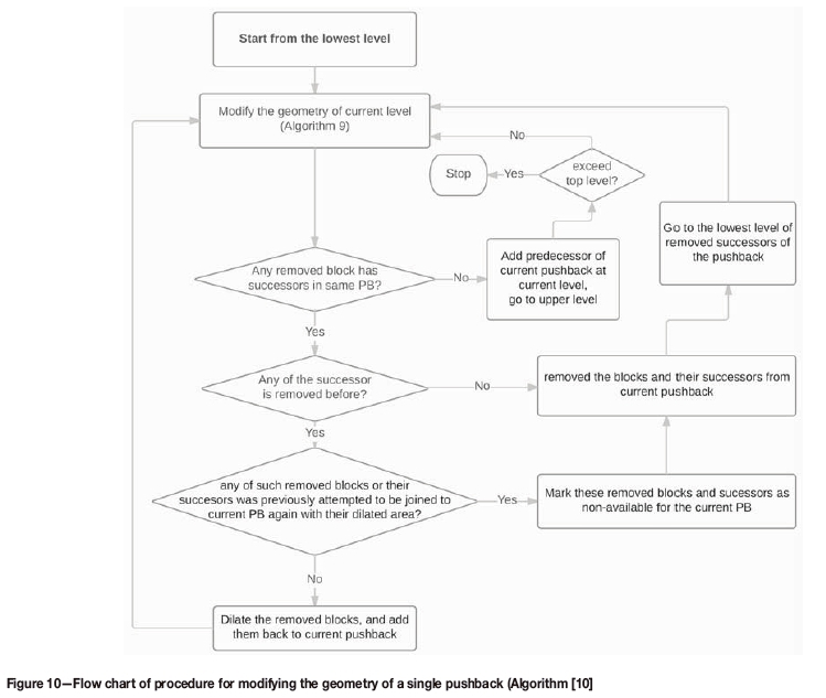
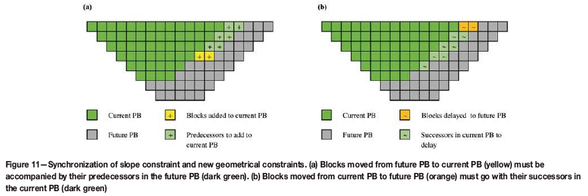
To create a pushback satisfying the three new geometrical constraints at all levels and keeping the slope constraints, we propose Algorithm [10], with the flow chart shown in Figure 10. The procedure essentially repeats the 'ModifyBenchGeometry' procedure (Algorithm [9]) level by level, from bottom to top. When generating the t^th pushback, these operations result in two effects: (1) delaying some blocks from pushback t to later, and (2) bringing some blocks forward to pushback t. Therefore, after the morphological operations, the precedence relationship should be accounted for. Specifically, if a block is brought forward to pushback t, its predecessors in future pushbacks should be moved to pushback t as well, in order to ensure the accessibility of the block (Figure 11a). Otherwise, if a block is delayed, its successors should also be delayed (Figure 11b), as the blocks at lower levels are no longer accessible. If any of its successors are delayed, the procedure will go back to the lowest level of the delayed block, and redo Algorithm [9]. Sometimes, the delayed successors may be recovered by the geometrical operations at these lower levels, thus a cycle can occur. When a cycle is detected, the delayed blocks are dilated and added back to pushback t. The dilation is repeated a few times if necessary to try to break the cycle. If after a few dilations the cycle remains, the blocks in question are expelled from pushback t and added to a Tabu list, which is sent to the geometric operators so as to prohibit appending these blocks again to pushback t.

Main algorithm: modified parametric maximum flow

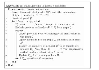
To achieve our goal of generating practical pushbacks with all geometrical constraints fulfilled, we need a high-level algorithm that utilizes Algorithm [10] to create multiple feasible pushbacks. We introduce Algorithm [11] for doing this. Since the structure of Algorithm [10] requires a pushback at earlier stages to be feasible, applying it on several nested pits simultaneously will not necessarily create multiple pushbacks with feasible geometry, nor guarantee satisfaction of resource constraints. Therefore, Algorithm [11] is designed to create pushbacks sequentially, from the first to last. When generating a new pushback, previous pushbacks are considered to be mined, so that modification only works on unplanned blocks. We use max-flow to create a parametric pit as an initial pit to be modified by Algorithm [10]. The modified pushback is then checked to assure the fulfillment of the production capacity constraints. A pushback that satisfied the constraints will be accepted; otherwise, it will be abandoned, then the price parameter will be adjusted and the max-flow and modification procedure repeated until the capacity requirement is met. The definition of resource constraints here can be very flexible, and the selection can depend on the specific application case. Here, for simplicity of description, we use only the ore tonnage constraint.

Algorithm [11] without geometrical modification (step 9) outlines a variant of the nested shells method, which is referred as 'successive max-flow' in the text above. This is similar to Whittle's nested shell solution in terms of selecting pit shells to match resource constraints. but works in an automatic way. We use it as a comparative method in following case studies.

 

Test results and discussion

The proposed algorithm is tested with two deposit models, one synthetic and one real. The goals of the test are to (1) evaluate the fulfillment of the new geometrical constraints in the created pushbacks, (2) analyse the variation of tonnage and size of pushbacks before and after geometrical modification, (3) assess the change of profit due to imposing new geometrical constraints, comparing with successive max-flow method, and (4) evaluate the computation time. The descriptions of testing data and design parameters are listed in Table I. The ultimate pits in the tests are created by a maximum flow algorithm and then modified by the geometric operators to ensure sufficient smoothness and enough width at pit bottom.

 

 

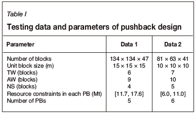
The first test data is from an artificial deposit created by FFTMA (Fast Fourier Transformation Moving Average) geostatistical simulation method (Ravalec, Noetinger, and Hu, 2000). The model contains 134 χ 134 χ 47 blocks. The unit block is 15 m χ 15 m χ 15 m. Pushback design uses the unique slope angle of 45° over the domain, and target width of 90 m, i.e. six blocks. Auxiliary width control parameter AW is 135 m (i.e. nine blocks). The smoothing factor NS adopts four blocks. The final pit is divided into five PBs. The tonnages of ore (blocks with positive profit) in each pushback are constrained to lie between 11.7 to 17.6 Mt (i.e. between 11 556 and 17 383 ore blocks at 3 t/m3). Note that the ore tonnage range is flexible and should be adjusted considering the capacity tolerance of processing plants and the possible use of one or more stockpiles.

The second test data is from a real copper mine; the name and location are undisclosed for confidentiality reasons. A part of the deposit was previously mined, and pushbacks need to be designed for the remaining material. The testing data consists of 81 χ 63 χ 41 blocks, with a block size of 10 m χ 10 m χ 10 m. The slope is 45° over the domain, the target width is 70 m, i.e. seven blocks wide. Auxiliary width control parameter AW is 100 m (i.e. 10 blocks). The smoothing factor NS is five blocks. The ore blocks are sent to a single mill. The mining production plan is divided into six periods. The tonnages of ore in each pushback are constrained to lie between 6.0 and 11.0 Mt (i.e. between 2000 and 3667 ore blocks at 3 t/m³).

Geometric constraints, NPV, and tonnage

For the calculation of NPV, we first create a simple block sequence in each pushback and then discount the value of each block according to its sequence number. The block sequencing mimics the actual mining sequence, with three levels of precedence: (1) the blocks in an earlier pushback precede those in later pushbacks; (2) in one pushback, the blocks on higher bench levels are extracted before those at lower levels; (3) on each bench, the blocks are mined from east to west. The discount period is the time required to mine a single block (ore or waste). The discount rate for each block is 1.259 χ 10-5. The UPit contains 37 858 blocks. The discount factor for the last block in the UPit is 1/(1 + 1.259 χ 10-5)37858 = 0.62. The (impractical) pushbacks generated by the nested shells method inside the same UPit are computed to provide a reference NPV. Note that these PBs do not respect the constraints of width, smoothness, and continuity. Hence, the reference NPV cannot be reached in practice. It is simply used as an indicator.

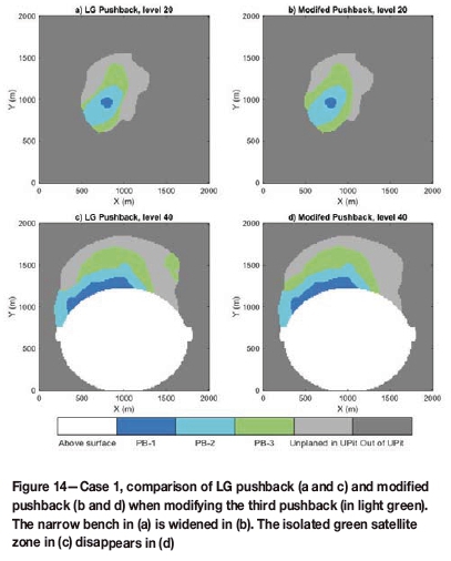
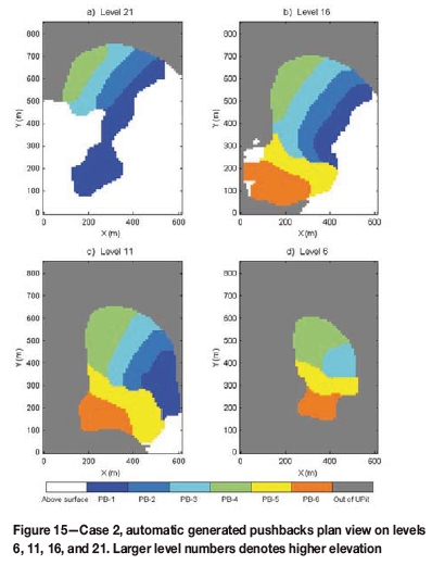
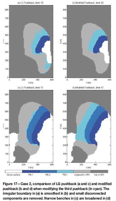
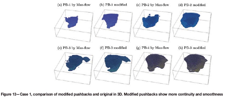
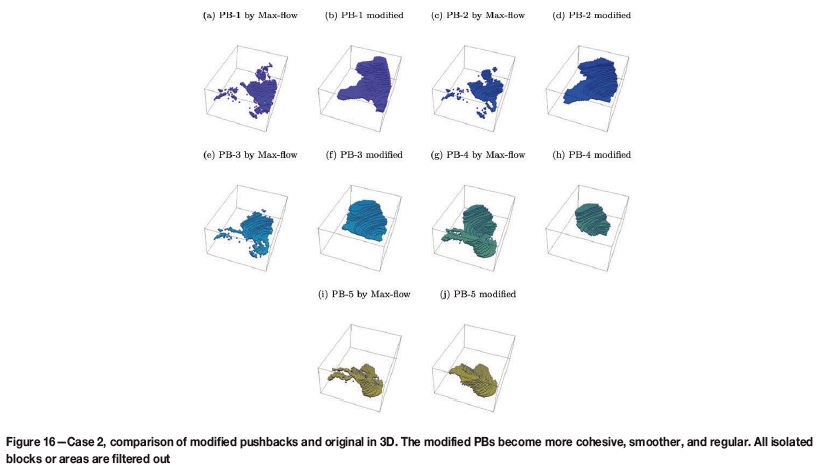
Figures 12 and 15 display the generated pushbacks on selected levels for the two cases. As is shown, the new geometrical constraints are all satisfied in the generated pushbacks. Most areas of the pushback benches are wider than the target minimum width. The pushback boundaries are regular and have smooth transitions with the pit of earlier periods. Also, each pushback has a single continuous component. In comparison, the pushbacks using the successive max-flow method do not show these desirable properties (shown in Figures 13 and 16). Those pushbacks are not mineable, as they present many isolated parts and are too irregular to be practical, especially in the real case no. 2. Figure 14 (for case 1) and Figure 17 (for case 2) show the change of the third pushback on different levels. In case 1, on level 20 (Figures 14a and 14b), the narrow bench is broadened to the target width, due to the effect of dilation. A similar effect can be seen on level 17 in case 2 (Figures 17c and 17d). On level 40 of case 1, the smaller isolated green areas of Figure 14c disappear in Figure 14d. A similar effect appears in case 2 level 10 (Figures 17a and 17b). Also, the larger cluster with irregular boundary in Figure 14a is smoothed.

 

 

 

 

 

 

Ore tonnages of modified pushbacks are plotted in Figure 18 along with the relative change in ore tonnage compared to the initial max-flow pit. Note that the capacity constraints are not applied on the max-flow pit as they are the solutions used to initiate our PB, which are the ones constrained by the processing capacity. The last pushback is not shown as it contains only the residual material, the ore tonnage for which does not cover an entire period. The application of the geometric operators globally enlarged the initial max-flow. For case 1, modified pushback ore tonnages are increased by 13% to 55% compared to the initial parametric pits obtained after 'mining' the previous PB. For case 2, the tonnage increase reaches 50% to 166%. The increase is mostly due to dilation applied at lower levels that requires appending a large number of predecessors at upper levels. One exception is the fourth pushback in case 2, where the tonnage is reduced by 46%. As shown in Figures 18a and 18c, the ore tonnages of the first five pushbacks are well within the capacity thresholds. The final pushback has insufficient tonnage feed, but this will not cause a practical problem, as it can be considered to be the production for a shorter period until the end of the mine life.

 

 

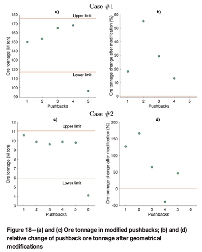
Figure 19 shows the NPV per ton of the different PBs. Note that the NPV per ton is computed over a substantially larger tonnage for the modified PB than for the successive max-flow PB, so it is difficult to directly compare these results. However, over the life of the mine, and then for the same UPit, the modified PB NPVs diminish compared to those obtained with the (non-mineable) successive max-flow PB, by 0.5% ($4.18 billion vs. $4.26 billion) for case 1, and by 7.3% ($685million vs. $739 million) for case 2. As expected, imposing more constraints reduces the NPV. Note, however, that in case 2, the 7.3% NPV reduction is due mostly to the first three PBs, where the successive max-flow PBs are clearly non-mineable (see Figure 16).

The NPV of the new method could be improved in a number of ways. First, the sequencing within each PB could be improved easily compared to the ad-hoc simple sequencing used here. Secondly, local search methods could be used to try to perturb the current PB definition by exchanging sets of blocks at the boundaries between the different PBs while still enforcing the geometric constraints to keep all the PBs mineable. This method is currently under investigation.

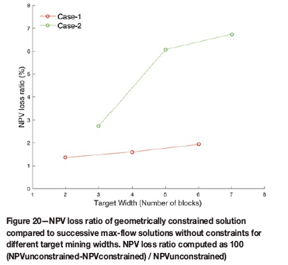
To analyse the sensitivity of the method to the new constraints, pushbacks are generated for a set of different mining widths. For case 1, the TW varies from two to six blocks; for case 2, it varies from three to seven blocks. To ensure that total value of the pit is same for comparison, the UPit for each case is created with the largest TW, i.e., six blocks for case 1 and seven blocks for case 2. We measure the NPV loss ratio relative to the successive max-flow method for these varying TWs, which is shown in Figure 20. It shows clearly that NPV decreases steadily with the increase of mining width.

 

 

In addition to the three new constraints introduced here, real-world pushback design also needs to take into account more requirements, such as ramp access and infrastructure constraints. These are detailed requirements that may impact the final pushback design on different scales. They are nevertheless difficult to measure in standard ways, unlike pit slope and mining width. Integrating the full set of design constraints and delivering automated designs is an area for further research.

Computational aspects

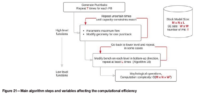
Figure 21 shows the main steps and associated variables in the proposed algorithm. Since the pushbacks are generated sequentially, the number of pushbacks scales linearly with the computation time. For the definition of a given pushback, the computing time for maximum flow depends on the spatial distribution of values in the block model. The application of geometrical constraints works bench-by-bench from bottom to top, but possibly with many ups and downs due to the removal of blocks on the upper level that have successors at lower levels in the same pushback. The computing time depends on the geometry of the pushback created by maximum flow, the complexity of the contour of already-mined zones, and the boundary of the ultimate pit.

The bench modification utilizes a series of morphological operations. Typically, the computational complexity of morphological algorithms is (MNW²) , where M and N are the dimensions of the block model in a horizontal plane, and W is the width of the structural element used in the operation. One can consider that between six and ten mining blocks usually suffice to create enough width for the equipment. Hence, the dominant terms for computing time are clearly the size of the deposit, M and N.

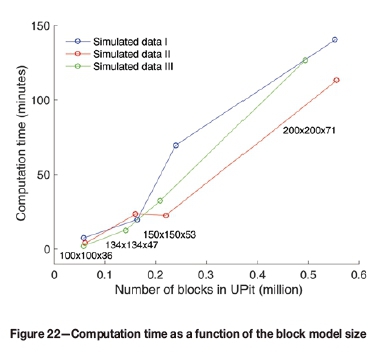
We used three simulated deposit of different sizes: 100 χ 100 χ 34, 134 χ 134 χ 47, 150 χ 150 χ 53, and 200 χ 200 χ 71. Figure 22 displays the computation time as a function of the size of the UPit for a fixed number of pushbacks. The design uses TW = 7 blocks. Tests were done on a laptop computer with Intel Core i5 2.5G CPU and 8 GB RAM. The programs were run in Matlab. Figure 22 shows that the program takes around 4 minutes to process a UPit with less than 100 000 blocks, and around 2 hours for a UPit with 550 000 blocks. Moreover, the computation time appears to globally scale quasi-linearly with the UPit size. This demonstrates that the algorithm is able to handle a medium-size block model in an affordable time, especially when compared to the time required for manual editing. Admittedly, processing a block model with more than 1 million blocks in the UPit would benefit from slight improvements to the current implementation of the method. One promising avenue is to use the more efficient implementation of morphological operations described in Dokládal and Dokládalová (2011), or simply to use a C++ compiled version or alike.

 

 

Conclusion

In this paper we propose a new algorithm to automatically generate mining pushbacks with practical geometries. The algorithm can manipulate the new geometrical constraints, including pushback bench and bottom width, smoothness, and continuity. A case study demonstrates that by reshaping the non-mineable initial pushbacks, one can obtain modified mineable pushbacks with marginal loss on the NPV value. The method is computationally efficient and has the potential to significantly contribute toward the automation of highly practical pushback designs.

 

Acknowledgments

This research was financed by NSERC Engage and Engage Plus Grants, Mitacs Accelerate, as well as Datamine Software Inc. and D. Marcotte NSERC research grant RGPIN-2015-06653. Two anonymous reviewers provided constructive suggestions for improving the draft.

 

References

Bai, X., Marcotte, D., and Simon, R. 2014a. A heuristic sublevel stope optimizer with multiple raises. Journal of the Southern African Institute of Mining and Metallurgy, vol. 114. pp. 427-434.         [ Links ]

Bai, X., Marcotte, D., and Simon, R. 2013b. Underground stope optimization with network flow method. Computers and Geosciences, vol. 52. pp. 361-371. https://doi.org/10.1016/j.cageo.2012.10.019        [ Links ]

Bai, X., Marcotte, D., and Simon, R., 2013c. Incorporating drift in long-hole stope optimization using network flow algorithm. Proceedings. of the 36th International. Symposium on Application of Computers and Operations Research in the Mineral Industry. (APCOM), Porto Alegre, Brazil. Costa, J.F., Koppe, J., and Peroni, R. (eds). Fundajao Luiz Englert, Porte Alegre. pp. 391-400. https://doi.org/10.13140/2.1.3534.6880        [ Links ]

Chandran, B.G. and Hochbaum, D.S. 2009. A computational study of the pseudoflow and push-relabel algorithms for the maximum flow problem. Operations Research, vol. 57, no.2. pp. 358-376. https://doi.org/10.1287/opre.1080.0572        [ Links ]

Chiles, J.-P. and Delfiner, P. 1999. Geostatistics: Modeling Spatial Uncertainty. Wiley.         [ Links ]

Consuegra, F.R.A. and Dimitrakopoulos, R. 2010. Algorithmic approach to pushback design based on stochastic programming: method, application and comparisons. Mining Technology, vol. 119. pp. 88-101. https://doi.org/10.1179/037178410X12780655704761        [ Links ]

Datamine. 2014. NPV Scheduler. The complete strategic mine planning system. http://www.dataminesoftware.com/npv-scheduler/        [ Links ]

Deraisme, J., de Fouquet, C., and Fraisse, H. 1984. Geostatistical orebody model for computer optimization of profits from different underground mining methods. Proceedings of the 18th APCOM Symposium.. London, UK. Institution of Mining and Metallurgy, London. pp. 583-590.         [ Links ]

Dokládal, P. and Dokládalová, E. 2011. Computationally efficient, one-pass algorithm for morphological filters. Journal of Visual Communication and Image Representation, vol. 22. pp. 411-420. https://doi.org/10.1016/jjvcir.2011.03.005        [ Links ]

Goldberg, A.V. and Tarjan, R.E. 1988. A new approach to the maximum-flow problem. Journal of the Associationfor Computing Machinery, vol. 35. pp. 921-940.         [ Links ]

Goodfellow, R. and Dimitrakopoulos, R. 2013. Algorithmic integration of geological uncertainty in pushback designs for complex multiprocess open pit mines. Mining Technology, vol. 122. pp. 67-77. https://doi.org/10.1179/147490013X13639459465736        [ Links ]

Hochbaum, D.S. 2008. The pseudoflow algorithm: a new algorithm for the maximum-flow problem. Operations Research, vol. 56. pp. 992-1009. https://doi.org/10.1287/opre.1080.0524        [ Links ]

Hochbaum, D.S. and Chen, A. 2000. Performance analysis and best implementations of old and new algorithms for the open-pit mining problem. Operations Research, vol. 48. pp. 894-914.         [ Links ]

Hopcroft, J. and Tarjan, R. 1973. Algorithm 447: efficient algorithms for graph manipulation. Communications of the Associationfor Computing Machinery, vol. 16. pp. 372-378. https://doi.org/10.1145/362248.362272        [ Links ]

Hustrulid, W. and Kuchta, M. 1995. Open Pit Mine Planning & Design: Fundamentals. Balkema.         [ Links ]

Juárez, G., Dodds, R., Echeverría, A., Guzmán, J.I., Recabarren, M., Ronda, J., and Vila-Echague, E. 2014. Open pit strategic mine planning with automatic phase generation. Proceedings of the Orebody Modelling and Strategic Mine Planning Symposium 2014. Australasian Institute of Mining and Metallurgy, Melbourne. pp. 147-154.         [ Links ]

Lerchs, H. and Grossmann, I.F. 1965. Optimum design of open-pit mines. Transactions of the Canadian Institute of Mining, Metallurgy, and Petroleum, vol. LXVIII. pp. 17-24.         [ Links ]

Marcotte, D. and Caron, J. 2013. Ultimate open pit stochastic optimization. Computers and Geosciences, vol. 51. pp. 238-246. https://doi.org/10.1016/jxageo.2012.08.008        [ Links ]

Meagher, C., Dimitrakopoulos, R., and Vidal, V. 2015. A new approach to constrained open pit pushback design using dynamic cut-off grades. Journal of Mining Science, vol. 50. pp. 733-744. https://doi.org/10.1134/S1062739114040140        [ Links ]

Nelis, G., Gamache, M., Marcotte, D., and Bai, X. 2016. Stope optimization with vertical convexity constraints. Optimization and Engineering, 2016, no. 4. pp. 1-20. https://doi.org/10.1007/s11081-016-9321-6        [ Links ]

Ravalec, M., Noetinger, B., and Hu, L. 2000. The FFT Moving Average (FFT-MA) Generator: An efficient numerical method for generating and conditioning Gaussian simulations. Mathematical Geology, vol. 32. pp. 701-723. https://doi.org/10.1023/A:1007542406333        [ Links ]

Serra, J.P. 1982. Image Analysis and Mathematical Morphology. Academic Press, New York.         [ Links ]

Stone, P., Froyland, G., Menabde, M., Law, B., Rasyar, R., and Monkhouse, P. 2004. Blasor - blended iron ore mine planning optimisation at Yandi, Western Australia. Proceedings of the International Symposium on Orebody Modelling and Strategic Mine Planning. Australasian Institute of Mining and Metallurgy, Melbourne. pp. 285-288.         [ Links ]

Whittle, D. 2011. Open-pit planning and design. SME Mining Engineering Handbook. Darling, P. (ed.), Society for Mining, Metallurgy and Exploration (SME) Inc., Littleton, CO. pp. 877-902.         [ Links ]

Whittle, J. 1998. Four-X user manual. Whittle Programming Pty Ltd, Melbourne.         [ Links ]

 

 

Paper received Mar. 2017
Revised paper received Feb. 2018

 

 

Appendix