AFRIROCK 2017 INTERNATIONAL SYMPOSIUM

 

Reassessing continuous stope closure data using a limit equilibrium displacement discontinuity model

 

 

D.F. Malan; J.A.L. Napier

Department of Mining Engineering, Faculty of Engineering, Built Environment & IT, University of Pretoria, South Africa

 

 

---

SYNOPSIS

Time-dependent closure data in deep hard-rock mines appears to be a useful diagnostic measure of rock behaviour. Understanding this behaviour may lead to enhanced design criteria and modelling tools. This paper investigates the use of a time-dependent limit equilibrium model to simulate historical closure profiles collected in the South African mining industry. Earlier work indicated that a viscoelastic model is not suitable for replicating the spatial behaviour of the closure recorded underground. The time-dependent limit equilibrium model available in the TEXAN code appears to be a useful alternative as it can explicitly simulate the on-reef time-dependent failure of the reef. A key finding in this paper is that the model gives a much better qualitative agreement with the underground measurements. For both the model and actual data, the rate of time-dependent closure decreases into the back area. Calibration of the constitutive model nevertheless led to some unexpected difficulties, and element size plays a significant role. It was also noted that the simulated closure is complex as it reflects the combined result of a number of elements failing at different times. The closure rate does not decay according to a simple exponential model. Explicit simulation of the fracture zone in the face appears to be a better approach to simulating the time-dependent behaviour in deep hard-rock stopes. The calibration of the limit equilibrium model is very difficult, however, and further work is required.

Keywords: stope closure, time-dependent deformation, limit equilibrium model, TEXAN code.

---

 

 

Introduction

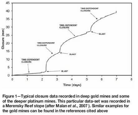
Several research studies have been conducted to investigate the use of continuous stope closure as a diagnostic measure of rock mass behaviour in deep gold mines of South Africa (e.g. Malan, 1995; Napier and Malan, 1997). The rock mass undergoes significant time-dependent deformation in some geotechnical areas and the closure data is useful for identifying different geotechnical areas and areas prone to face-bursting (Malan et al. 2007 ). The value of continuous closure measurements was also demonstrated for the platinum industry. An example is shown in Figure 1 to illustrate the significant 'creep' component recorded in some of the areas. For the gold mines, it was proposed that the data may be useful to identify remnants that can be safely extracted. A difficulty faced in these early studies was that no numerical tool could simulate the time-dependent rock mass behaviour on a stope-wide scale. It was hypothesised that the time-dependent behaviour in the hard-rock gold mines is caused by time-dependent fracturing and other inelastic processes, such as gradual slip on parting planes. In the platinum mines, the face fracturing is less intense and the behaviour is most likely dominated by the time-dependent failure of the crush pillars. The commonly used elastic modelling programs cannot simulate this behaviour and the simulated convergence is simply a function of the mine geometry, depth, and elastic constants. The analytical viscoelastic models that were derived for the previous studies could not be used for complex geometries and the elasto-viscoplastic finite difference models were limited to 2D and to a small number of mining steps (Malan, 1999). Recent studies have indicated that a limit equilibrium displacement discontinuity model with a time-dependent failure criterion may be useful for simulating on-reef time-dependent failure processes on a mine-wide scale (Napier and Malan, 2012, 2014). This paper explores the use of this model in the TEXAN code to simulate the historical time-dependent closure measurements.

 

 

 

Case study of measurements in a deep Venterdorp Contact Reef (VCR) stope

In 1997, the authors were involved with measurements conducted in the W3 updip panel in the 87/49 longwall at a mine in the Carletonville area. These particular measurements were valuable as they indicated that care should be exercised when using a viscoelastic model when simulating the time-dependent closure. The layout of the area is shown in Figure 2. Five closure instruments were installed simultaneously in different positions to investigate the effect of measurement position on the rate of time-dependent closure.

 

 

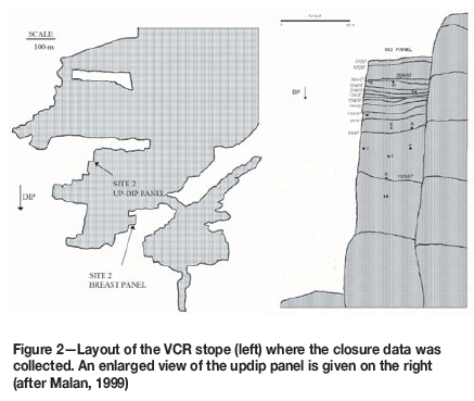
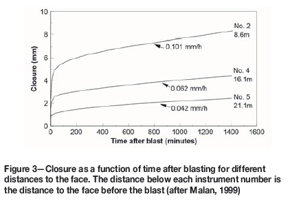
Figure 3 illustrates the increase in closure after a blast on a specific day. All three measurements in the graph apply to the same blast, so the differences are only a function of the measurement position. This data illustrates the decrease in rate of time-dependent closure as the distance to the face increases.

 

 

A further important characteristic of the data is that the rate of time-dependent closure appears to be constant in the short term, but it gradually decreases when there is no blasting or seismic activity. This is illustrated in Figure 4. This particular data-set was obtained for the site in Figure 2 during a period when there was no mining activity for several days. The time-dependent closure can be approximated by an exponential decay function of the form:

 

 

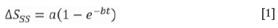
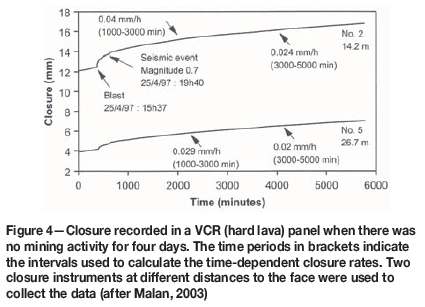
where a and b are parameters and t is time. The time-dependent closure for station no. 2 in Figure 4 after the seismic event was plotted in Figure 5 together with the model given in Equation [1]. The parameters used to obtain this fit were a = 3.85 mm and b = 0.015 h-1.

 

 

The problem with viscoelastic theory

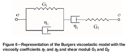
To simulate the time-dependent deformations recorded in tabular excavations, a viscoelastic approach was investigated (Malan, 1999). A two-dimensional closure solution for a parallel-sided tabular excavation in a viscoelastic medium was derived for this study. In linear viscoelastic theory, complex strain-time behaviour can be described by various combinations of two principal states of deformation: elastic behaviour and viscous behaviour. The historical use of different viscoelastic models to simulate the creep of rocks is given in many papers {e.g. Ryder and Jager, 2002). Malan (1999) assumed a Burgers model to describe the time-dependent behaviour shown in Figure 1. This model is shown in Figure 6. The complete viscoelastic closure solution when assuming this model is given in Malan et al. (2007).

 

 

Using this approach, a good fit with data over a short period of time (e.g. 1 day) could be obtained. Problems were nevertheless encountered when attempting to calibrate the model at various distances from the mining face (e.g. Figure 3). These problems arise as the viscoelastic model predicts that the rate of time-dependent convergence increases towards the centre of the stope. This can be shown by taking the time derivative of the viscoelastic closure solution. For time t→ ∞, the rate of convergence is given by (see Malan, 1999):

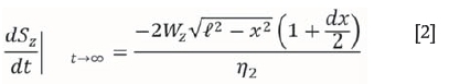
where

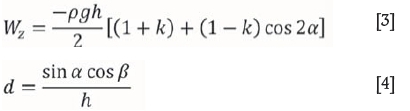
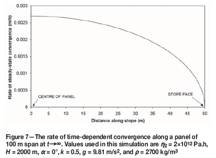
and S_zis the stope closure, is the span of the stope, ρ is the density of the rock, x is the position in the stope relative to the centre, g is the gravitational acceleration, h is the depth below surface, k is the ratio of horizontal to vertical stress, a is the dip of the reef, β is the angle between the x-axis and the dip, and t is time. The Burgers viscosity coefficient η₂ is defined in Figure 6. As t→ ∞, the rate of convergence is therefore only a function of geometric parameters, stress magnitude, and the viscoelastic parameter η₂. This is intuitively expected from Figure 6.

The rate of time-dependent convergence (Equation [2]) is plotted as a function of the position x in Figure 7. The rate of convergence is highest in the centre of the stope, and reduces to a value of zero at the stope face. This can be compared to the data collected in the mining stope (Figure 3), illustrating the opposite trend, where the rate of time-dependent closure decreases with increasing distance from the stope face. Additional data from the experimental site is given in Figure 8.

 

 

 

 

A further problem with the Burgers model is that it predicts that the rate of time-dependent closure remains constant. For t→ ∞, Equation [2] does not tend to zero, but indicates a constant rate of convergence. In contrast, Equation [1] can be differentiated to give the rate of time-dependent convergence for the actual data as:

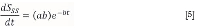
Equation [5] indicates that the rate of time-dependent closure tends to zero as t→ ∞.

 

A proposed time-dependent limit equilibrium model

As an alternative to the viscoelastic model, a time-dependent limit equilibrium model built into the displacement discontinuity code TEXAN was used to investigate the closure behaviour described above. A description of the TEXAN code and the limit equilibrium model is given by Napier and Malan (2012, 2014). Following this approach, the fracture zone surrounding the excavations is simplified as the model restricts failure to the on-reef plane. A key feature of the model is that the intact rock strength is differentiated from the residual strength according to specified intact and residual failure strength envelopes. The strength of the intact seam or reef material ahead of the stope face is assumed to be defined by a linear relationship of the form

where and mi are the intercept and slope parameters respectively, as is the average seam-parallel confining stress, and a_nis the seam-normal stress component. Once a point in the seam fails, the strength parameters are postulated to decrease immediately to values σί° and m₀, which define an initial limit stress state in which there is a fixed limit equilibrium relationship between a_nand a_sof the form

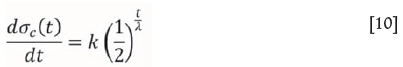
The limit strength parameters are then assumed to decay towards residual values and m_j. The strength values oc(t) and m( t) at an elapsed time t after failure, are defined according to the relationships:

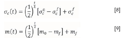
where λ is a half-life parameter. The limit stress components on and as at a given seam or reef position and time t are then given by an appropriate equation of similar form to Equation [6]:

The reef-parallel (or seam-parallel) stress is determined by setting up an averaged force balance at each point in the fracture zone, which depends on the effective fracture zone height H and on the contact friction coefficient μι between the broken material and the intact rock enclosing the fracture zone (Napier, 2016). It is apparent that the distribution of the limit stress values will in general depend on the distribution of failure times at all points in the fractured material, and consequently depends in a complex evolutionary manner on the planned mining sequence and extraction rate. A given mining problem must therefore be solved in a series of timesteps which include mining increments that are scheduled at appropriate time-step intervals. The problem time-scale will be determined essentially by the chosen half-life parameter, λ. A novel solution algorithm has been developed to calculate the distribution of stress components a_nand a_s, as well as the overall extent of the fracture zone arising in each simulated time step. A detailed description of this procedure is given by Napier (2016).

 

Simulation of time-dependent closure

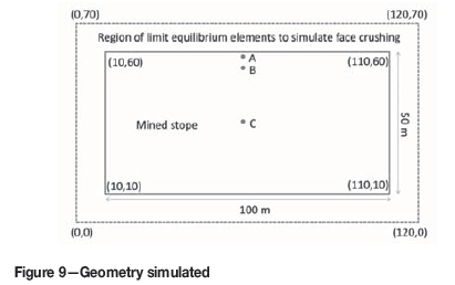
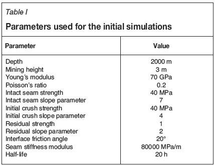
The simplified geometry shown in Figure 9 is used to illustrate the characteristics of the time-dependent limit equilibrium model. This is a stope of size 100 m χ 50 m situated at a depth of 2000 m. The stope is surrounded by a region of elements which assume the constitutive behaviour described by Equation [8] to [10] once failure is initiated. Closure profiles were recorded at points A, B, and C. These measurement positions varied slightly depending on the element sizes used, but for 1 m elements, the distances to the excavation face were A = 0.5 m, B = 4.5 m, and C = 24.5 m. The model parameters are given in Table I. These parameter values are assumed and need to be calibrated in future.

 

 

 

 

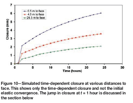
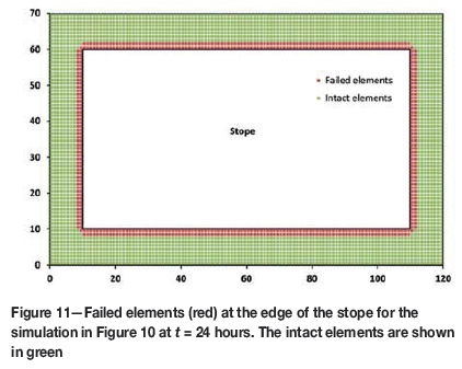
The first simulation attempted to replicate the underground closure behaviour shown in Figure 3. The simulated results are shown in Figure 10 and the time-dependent nature of the closure is clearly visible. Note that the rate of time-dependent closure decreases into the back area of the stope, similar to the underground observations. This model is therefore clearly an improvement on a simple viscoelastic approach, which could not replicate this behaviour. Figure 11 illustrates the failed limit equilibrium elements (red) and the intact elements (green).

 

 

 

 

Effect of grid size

Although the results in Figure 10 look encouraging, it was noted during further simulations that the grid size and sequential failure of the elements affect the simulated closure profiles. An example is illustrated in Figure 12. The parameters for these simulations were identical to those in Table I, except for the red closure profile where it was specified that the initial crush slope parameter was 7 (similar to the intact slope parameter). Note the jumps in closure. The mining geometry remains constant during these jumps, which are caused by the sequential failure of the next row of limit equilibrium elements. As the grid consists of square elements and the geometry is regular, the failure of the elements occurs row by row in an organized pattern. A particular row is activated and a jump in closure occurs as the stress is transferred to the solid ground according to the model in Equations [8] and [9]. The next row eventually fails and the process repeats. Figure 13 illustrates the extent of the failed zone after 168 hours. The number of rows of elements activated corresponds to the number of jumps in closure visible in Figure 12. The first part of Figure 12 is enlarged in Figure 10, and this explains the anomaly at the beginning of the curve in Figure 10. A possible solution would be to reduce the element size as shown in Figure 14. For smaller elements, the jumps in closure are more frequent, but smaller in magnitude. This improves further if the intact strength and initial crush strength are identical (not shown here).

 

 

 

 

 

 

Partial element fracturing

Figure 15 depicts a conceptual view of the stress profile transition between the edge of the fractured rock at position L and the adjacent intact material. (Figure 15 may be considered to represent a local section profile that is aligned in the normal direction to the fracture zone edge.) The basic solution algorithm (Napier 2016) that has been developed to infer the transition from an intact state to a failed state is accurate only to the resolution of the element grid size, g. A revised scheme has been developed more recently to predict the intermediate position L of the fracture front between successive collocation points, as shown in Figure 15. Once the front position L has been estimated, a fractional subelement with an appropriate shape, centre position, and self-effect coefficient is constructed within the partially fractured element to determine the effective displacement discontinuity strain and reef-normal stress in the element. A current restriction on the new algorithm is that the controlling rock strength parameter ratios must be such that

 

 

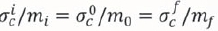
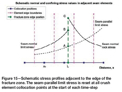
Figure 16 shows a comparison between the proposed partial element fracturing scheme and the existing algorithm for the rectangular excavation layout shown in Figure 9. The incremental closure profiles are measured at point A in Figure 9. It is apparent that the partial fracturing algorithm allows the fracture zone to extend in more continuous steps than in the base case, where an abrupt failure transition occurs after time step 42 (see the bottom curve in Figure 16). It is also observed that the fracture zone extent increases over a greater distance in the case where partial element fracturing is included.

 

 

The upper curve in Figure 16 shows the incremental closure profile that would arise in the case of a plane strain parallel-sided excavation with a nominal span of 50.0 m and with a very fine element mesh size g of approximately 0.0909 m. This case was evaluated to determine approximately the asymptotic effect of reducing the element grid size. It should be noted that the effective layout depth in the plane strain case was reduced from 2000 m to 1760 m (a factor of approximately 0.88) to compensate for the infinite lateral span of the parallel-sided panel, compared to the 100.0 m lateral span in the rectangular excavation (see Figure 9). Figure 16 shows that the fine grid behaviour is approximately replicated by the partial element fracturing algorithm, but that the underlying fracture front transitions are still somewhat dependent on the element mesh size.

Figure 17 shows the incremental closure profiles that are obtained for the rectangular excavation shown in Figure 9 following a mining step of 1.0 m at the upper face after timestep 72. The profiles are monitored at points A, B, and C shown in Figure 9. Figure 17 illustrates the progressive decrease in the incremental rate of closure as the distance from the mining face is increased. The strength parameters used in the partial element fracturing results in Figure 16 and Figure 17 are as follows:

 

 

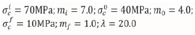
The remaining parameters are as summarized in Table I.

 

Calibration of the half-life parameter

The rate of change for the underground closure data shown in Figure 4 is approximated by the exponential decay model in Equation [5]. For the numerical model, the decay of the strength of the failed limit equilibrium elements gives rise to the stress transfer and the simulated time-dependent closure. It is therefore postulated that the actual underground closure data can be used to calibrate the half-life parameter of the numerical model. If Equation [8] is differentiated, the rate of strength decrease for a failed limit equilibrium element is:

where

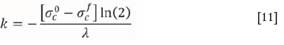
It is known that and (see Equation [5]) are equivalent formulae to describe exponential decay, and it can be shown that:

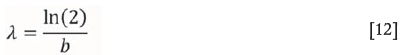
For Figure 5, it was found that b = 0.015 h-1 gives a good fit to the data, and from Equation [12] it follows that λ = 46.2 hours. Time-dependent closure data from the platinum mines fitted with the model described in Equation [1] is also given in Roberts et al. (2006). Table II illustrates the data currently available for which the b parameter was calculated and the corresponding value of λ is given.

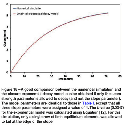
Care should be exercised for the two sites in Table II with calibrated λ values greater than a hundred. The hangingwall at these two sites was unravelling. This caused the large ongoing time-dependent closure. In contrast, the failure processes and stress transfer ahead of the face or in pillars dominated at the other two sites. As the current implementation of the model in TEXAN makes provision for both the seam strength and seam slope parameter to undergo exponential decay, care should be exercised when calibrating the model using the λ values in Table II. To illustrate this, a model similar to Figure 9 with element sizes of 2 m and just one row of limit equilibrium models at the edge of the stope was used. The resulting time-dependent closure curve is shown in Figure 18. The parameters were similar to those in Table I, with minor changes as indicated in the figure caption. Note that a single row of elements that fail simultaneously where only the seam parameter (and not the slope parameter) is allowed to decay, also results in a simple exponential decay for the closure. In contrast, if both parameters are allowed to decay using the same half-life value, more complex behaviour is the result and the fit of the simulated closure with Equation [1] is not good.

 

 

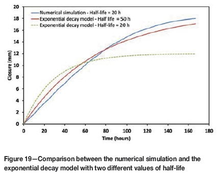
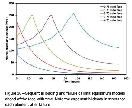
To complicate matters, the sequential activation of a larger number of limit equilibrium elements at different times leads to a simulated closure profile that differs from the simple exponential decay model. To illustrate this, the model in Figure 9 was simulated with 0.5 m element sizes. The parameter values in Table I were assumed, except that all three slope parameters were assigned a value of 4. The time-dependent closure between t = 1 h and t = 168 h is plotted in Figure 19. The numerical model assumed a half-life of 20 h. The exponential decay model with the equivalent b-value gives a very poor fit. It appears that the sequential activation of the elements (Figure 20) results in a closure profile that cannot be simulated with a simple exponential model.

 

 

 

 

 

Conclusions

Time-dependent closure data in deep hard-rock mines appears to be a useful diagnostic measure of rock behaviour.

Understanding this behaviour may lead to enhanced design criteria and modelling tools. This paper investigates the use of a time-dependent limit equilibrium model to simulate historical closure profiles collected in the South African mining industry. Earlier work indicated that a viscoelastic model is not suitable for replicating the spatial behaviour of the closure recorded underground. The time-dependent limit equilibrium model available in the TEXAN code appears to be a useful alternative, as it can explicitly simulate the on-reef time-dependent failure of the reef seam. A key finding in this paper is that the model gives a much better qualitative agreement with the underground measurements. For both the model and actual data, the rate of time-dependent closure decreases into the back area. Calibration of the constitutive model nevertheless led to some unexpected difficulties, and element size plays a significant role. It appears that this problem can be addressed to some extent by introducing a sub-element construction algorithm that allows the moving edge of the fracture zone to be simulated in partially fractured elements. Further work on this procedure is required.

It was noted also that the simulated closure profile is complex as it reflects the combined result of a number of elements failing at different times. The closure rate does not decay according to a simple exponential model. In conclusion, explicit simulation of the fracture zone in the face appears to offer a better approach to describe the observed time-dependent behaviour in deep hard-rock stopes. The calibration of the limit equilibrium model half-life decay parameter requires additional field measurements in different geotechnical areas.

 

References

Malan, D.F. 1995. A viscoelastic approach to the modelling of transient closure behaviour of tabular excavations after blasting. Journal of the South African Institute of Mining and Metallurgy, vol. 95. pp. 211-220.         [ Links ]

Malan, D.F. 1999. Time-dependent behaviour of deep level tabular excavations in hard rock. Rock Mechanics and Rock Engineering, vol. 32, no. 2. pp. 123-155.         [ Links ]

Malan, D.F. 2003. Guidelines for measuring and analysing continuous stope closure behaviour in deep tabular excavations. Safety in Mines Research Advisory Committee (.SIMRAC), Johannesburg. August 2003.         [ Links ]

Napier, J.A.L. 2016. Application of a fast marching method to model the development of the fracture zone at the edges of tabular mine excavations. Proceedings of the 50th US Rock Mechanics/Geomechanics Symposium, Houston, Texas, 26-29 June, 2016. American Rock Mechanics Association.         [ Links ]

Napier, J.A.L. and Malan, D.F. 1997. A viscoplastic discontinuum model of time-dependent fracture and seismicity effects in brittle rock. International Journal of Rock Mechanics and Mining Sciences & Geomechanics Abstracts, vol. 34. pp. 1075-1089.         [ Links ]

Napier, J.A.L. and Malan, D.F. 2012. Simulation of time-dependent crush pillar behaviour in tabular platinum mines. Journal of the Southern African Institute of Mining and Metallurgy, vol. 112. pp. 711-719.         [ Links ]

Napier, J.A.L. and Malan, D.F. 2014. A simplified model of local fracture processes to investigate the structural stability and design of large-scale tabular mine layouts. Proceedings of the 48th US Rock Mechanics/Geomechanics Symposium, Minneapolis, MN, 1-4 June, 2014. American Rock Mechanics Association.         [ Links ]

Roberts, D.P., Malan, D.F., Janse van Rensburg, A.L., Grodner, M., and Handley, R. 2006. Closure profiles of the UG2 and Merensky reef horizons at various depths, using different pillar types, in the Bushveld Complex. Final report SIM040207. Safety in Mines Research Advisory Committee (SIMRAC), Johannesburg.         [ Links ]

Ryder, J.A. and Jager, A.J. 2002. A Textbook on Rock Mechanics for Tabular Hard Rock Mines. Safety in Mines Research Advisory Committee (SIMRAC), Johannesburg.         [ Links ] ♦

 

 

This paper was first presented at the AfriRock 2017 International Symposium, 30 September -6 October2017, Cape Town Convention Centre, Cape Town.