PAPERS OF GENERAL INTEREST

 

Numerical and physical modelling of tundish slag entrainment in the steelmaking process

 

 

A. Mabentsela; G. Akdogan; S. Bradshaw

Department of Process Engineering, Stellenbosch University, Stellenbosch, Cape Town, South Africa

 

 

---

SYNOPSIS

Physical and numerical modelling methods were followed to identify mechanism(s) for tundish slag entrainment in a bare tundish and one with a flow control device (FCD).
The physical and numerical models made use of water and paraffin to model steel and slag respectively. Observations from the physical model showed that the steel-slag interface remains immobile in both cases. Entrained paraffin formed droplets approximately 1 mm in diameter. Results from both models (numerical and physical) showed that in both cases (bare and FCD case), areas of high entrained slag concentration exist near the inlet region. The entrained slag concentration decreases towards the tundish endwalls.
Flow patterns and velocities tangential to the steel-slag interface from the numerical model showed that slag entrainment in both the bare tundish and tundish with a FCD possibly takes place via two mechanisms. First, the slag moves across the steel-slag interface via mass transfer; secondly small velocities tangential to the interface at depths greater than 10 mm below the interface carry the already 'entrained' slag into the bulk steel phase. These tangential flow patterns are dominant in the inlet region, hence the high concentration of entrained slag in this region.

Keywords: tundish slag entrainment, tundish slag behaviour, numerical modelling, slag shearing.

---

 

 

Introduction

The tundish serves as the last metallurgical vessel through which steel passes before solidifying in the moulds. It is in the tundish that the last traces of non-metallic inclusions should be removed, otherwise the inclusions carry over to the moulds and cause defects in the steel product. In the tundish, the slag is less dense than the melt and thus resides on the top of the melt. The slag provides a sink into which the non-metallic inclusions float to and dissolve. The slag also protects the melt from air and heat loss. However, when slag is entrained in the melt as a result of increased turbulence or shearing at the steel-slag interface, slag can become a source of non metallic inclusions.

Numerous studies on flow patterns in the tundish have been carried out since the introduction of the tundish. These studies were aimed at improving the flow characteristics in the tundish (Chattopadhyay, Isac, and Guthri, 2010; Cloete, 2014; Jha, Dash, and Kumar, 2001; Jha, Rao, and Dewan, 2008; Kumar, Koria, and Mazumdar, 2007; Kumar, Mazumdar, and Koria, 2008; Mazumdar and Guthri, 1999; Sahai and Emi, 1996; Sahai and Burval, 1992; Tripathi and Ajmani, 2011). These studies have led to the use of flow control devices (FCDs) to increase the melt residence time in the tundish and provide surface-directed flow so as to assist with inclusion removal. FCDs include dams, weirs, baffles, and turbulence inhibitors. It is now generally understood that any tundish without a FCD suffers from poor inclusion removal as a result of too short a melt residence time in the tundish (Mazumdar and Guthri, 1999).

Due to the opaqueness of the steel melt and the elevated operating temperature (1600°C) in the tundish, the abovementioned studies were carried out using a combination of physical models, otherwise known as 'cold models', and numerical models. Physical models involve the use of reduced-scale water models where water is used to represent the steel melt. Numerical models involve using computational fluid dynamics packages to model the melt flow in the tundish. When used together, the physical model can be used to verify numerical model results. Once verified, the numerical model can then be adapted without the need of a physical model. This significantly reduces the costs of exploring new designs and also saves time.

The flow behaviour studies that have led to the use of FCDs were done using both physical and numerical models. In most of these studies, the researchers were only concerned with the melt phase, i.e. how the FCD affects the melt residence time. Most researchers opted to use only water in their physical and numerical models (Chattopadhyay, Isac, and Guthri, 2010; Cloete, 2014; Kumar, Mazumdar, and Koria, 2008; Mazumdar and Guthri, 1999; Sahai and Emi, 2008). As a result there is little or no information on how the FCDs affect the slag layer. This is evident in the lack of mentions of slag entrainment as a result of the use of FCDs in the review of two decades of work (1979 to 1999) by Mazumdar and Guthri (1999). In a more recent review of work on tundish technology from 1989 to 2009, Chattopadhyay, Isac, and Guthri (2010) noted the lack of research on how FCDs affect the slag phase, and pointed out the lack of both physical and numerical models to predict tundish slag entrainment. There is, therefore, a general lack of understanding on how tundish slag is entrained and how FCDs affect the slag layer.

Following from the above, the purpose of this study was to numerically and physically investigate tundish slag behaviour in a bare tundish and a tundish with a FCD device.

The objectives of this study are to:

► Use physical modelling techniques to study the behaviour of tundish slag in a bare tundish and in a tundish with a FCD

► Develop a numerical model that can predict tundish slag behaviour in both a bare tundish and a tundish with a FCD

► Identify, using the physical model and the numerical model, a mechanism (or mechanisms) for slag entrainment in a bare tundish and a tundish with a FCD

► Make recommendations based on the findings.

 

Slag entrapment mechanism

Entrainment of tundish slag into the steel melt can occur via vortexing, high-velocity flow that shears the slag at the slag-steel interface, and turbulence at the slag-steel interface (Hagemann et al., 2013).

Apart from high velocities at the interface, some authors have reported slag entrainment in slow steel melt velocity zones. This is thought to be caused by Kelvin-Helmholtz instability, which arises when two streams of fluid with different densities flow past one another. The presence of shear stress leads to instability, which causes the growth of waves which later roll into small vortices (Solhed and Jonsson, 2003). Slag entrainment can also occur as a result of Marangoni flow or by mass transfer across the interface. In Marangoni flow, the slag movement into the steel phase and vice versa is caused by local gradients of the interfacial tension caused by chemical reactions (Hagemann et al., 2013), while in the mass transfer method, slag and steel move across the interface due to low concentrations of the two fluids across the interface.

► Vortexing-Nagaoka et al. (1986) studied the effect of bath level on slag entrainment via vortex formation. They concluded that vortexing occurs during melt transfer to the mould when the bath level inside the tundish is low. Vortexing can therefore be controlled by controlling the bath level in the tundish. It is well known in the steelmaking industry that melt transfer during low bath level causes vortex formation, which leads to slag carrying over to the mould

► 5/eartog-Entrainment of a lighter phase into a heavy phase via shearing starts with finger-like protrusions of the lighter phase into the heavy phase. This fingering phenomenon can be described in terms of Taylor-Saffman instability, which occurs when a fluid of different density and viscosity relative to the second fluid pushes down on the second fluid. Feldabauer and Cramb, (1995) studied the entrainment of slag in the casting mould using Taylor-Saffman instability. They commented that the instability depended on interfacial tension, viscosity, and inertial energy exerted by the denser phase. The actual entrainment at the tip of a less dense protrusion into the denser phase is a function of the deforming stress exerted by the denser phase and the counteracting interfacial tension between both phases. The detachment of a droplet of the 'lighter' phase into the 'heavier' phase was further studied in a Couette device and four rollers, where the density ratio of the two fluids was unity (p%_eavy/p_ghter). The detachment of the lighter fluid into the heavier fluid was found to be a function of the viscosity ratios of the fluids used (Nheavy/N_lighter) and the dimensionless critical number, known as the critical capillary number (Hagemann et al., 2013). Hagemann et al. extended this research by studying the effect of the kinematic viscosity ratio of the two fluids (vigher/v_ieavy) on the critical capillary number (Ca*). They used a water model with a rotating roller to generate shear stress at the interface. Different silicon oils were used to represent the slag layer. In their studies the following definitions applied.

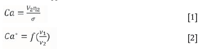
where V₂is the tangential velocity of the heavier phase below the interface, η₂the molecular viscosity of the heavier phase, a the interfacial tension between the two phases, v₁the kinematic viscosity, of the lighter phase, and v2₁the kinematic viscosity of the heavier phase Hagemann et al. (2013) showed that the critical capillary number for slag entrainment is a function of the ratios of kinematic viscosities, given by:

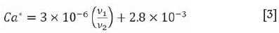
According to the above equation, increasing the ratio of kinematic viscosities of a system should raise the critical capillary number and thus reduce the chances of entrainment. If the capillary number of the system, calculated by Equation [1], is below the critical capillary number of that particular system no entrainment of slag will occur.

Hagemann et al. (2013) went on to study the effect of the slag layer thickness on the critical capillary number needed for slag entrainment to occur via shearing. They found that the slag layer thickness has no effect on the entrainment of slag resulting from shear stress at the interface.

A numerical study by Solhed, Jonsson, and Jonsson (2008) showed that slag entrainment in a one-strand bare tundish was caused by shearing at the interface.

They commented that shearing was caused by a recirculating flow in the inlet region. They also showed that the highest entrained slag concentration was in the region behind the inlet. However, Solhed, Jonsson, and Jonsson (2008) did not do any mathematical investigation to establish which of the mechanisms identified above was responsible for the slag entrainment they noted. Moreover, they did not consider FCDs and their effect on slag entrainment.

Harman and Cramb (1996) studied the size of the entrained slag droplets formed via shearing of the slag layer, using a water model. They noted that the first entrained slag droplet is the largest. They noted that the size of this droplet can be estimated by Equation [4].

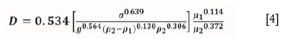
where D is the diameter of droplet, a the interfacial tension, g the gravitational acceleration, p₂the density of steel, pj the density of slag, μ₁the molecular viscosity of slag, and μ₂the molecular viscosity of water Hagemann et al. (2013) also studied the size of 'slag' droplets entrained via shearing at the interface using clod models. They found that the estimated droplet sizes were of the same order of magnitude as those of Harman and Cramb (1996). However, it is rather strange that they attempted to study the entrained droplet size with respect to changes in the kinematic viscosity ratio of the two fluids, when the empirical equation given by Harman and Cramb (1996) shows that the relationship between the droplet size and the viscosity ratio of the two fluids is not linear, and that it varies independently of each viscosity ratio.

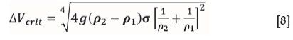
► Kelvin-Helmotz instability-Kelvin-Helmholtz instability takes place when two inviscid, irrotational fluids of different densities separated by a flat interface move at different tangential velocities (Hibbeler and Thomas, 2010). The instability and entrainment of slag takes place when the difference between the velocities of the two fluids exceeds a critical velocity difference given by:

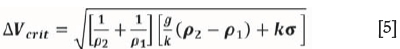
where ΔV_rcrit is the critical tangential velocity difference between steel and the slag, /¾ the density of steel, p₁the density of the slag, g the gravitational acceleration, a the interfacial tension between steel and slag, and k the angular wave number of small perturbation on the interface with wavelength λ.

The minimum wavelength at which Kelvin-Helmholtz instability takes place in nature is given by:

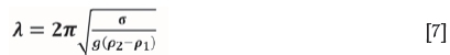
This gives rise to the minimal critical velocity at which Kelvin-Helmholtz instability takes place, which is given by:

Milne-Thomson (1968) extended Kelvin-Helmholtz instability to include finite fluid depth, but neglected the effect of viscosity and interfacial tension, yielding:

 

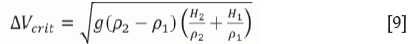
where H₁and H₂are the thickness of the slag layer and the steel melt layer respectively.

Iguchi and co-workers confirmed this using physical experiments that involved a rotating roller under water and oils. They found that the above equation is valid for low-viscosity and low-frequency disturbances where surface tension is not important or can be neglected (Iguchi et al., 2000).

► Turbulence at the interface-Turbulence at the steel-slag interface is caused by excessive surface-directed flow of the melt to the slag layer as a result of the flow reflecting from the bottom of the tundish or as a result of the improper use of FCDs. Too much surface-directed flow leads not only to slag entrainment but also to balding of the slag layer. In the latter case, the surface-directed flow is so high that it pushes the slag away and causes the melt to be exposed to air (Hibbele and Thomas, 2010).

► Marangoniflow-Exchange reactions, such as the oxidation of dissolved aluminium, that take place at the interface reduce the local interfacial tension between steel and slag and thus increase the system's capillary number. If the system's capillary number is increased past its critical value, then emulsification can occur even at low melt velocities. Similar to the exchange reactions at the interface, bubbling of argon from the bottom of the tundish decreases the local interfacial tension between steel and the melt, thus leading to slag entrainment even at low melt velocities (Hibbele and Thomas, 2010).

► Gas bubbling-Gas bubbling is often used in tundishes to promote flotation of inclusions. The gas of choice is argon due to its inertness. Gas injection may, however, lead to slag entrainment when the gas bubbles rupture at the upper slag layer. The bubbles rise due to buoyancy, they penetrate the slag layer, and once they reach the surface of the slag layer, they rupture, causing small slag droplets to enter the steel phase ((Hibbele and Thomas, 2010). Apart from this, as noted, bubbles bursting at the steel-slag interface also induce Marangoni flow.

► Mass transfer across the interface-Although not well documented in literature as a mechanism for slag entrainment, mass transfer across the steel-slag interface could possibly lead to low concentrations of slag in the steel phase and low steel concentrations in the slag phase. In a summary of model studies on slag entrainment mechanisms in gas-stirred ladles, Senguttuvan and Irons (2013) commented that entrainment of slag/steel across the steel-slag interface substantially increases the mass transfer rate across the interface. They go on to comment that identification or characterization of entrainment has been limited to establishing the conditions for entrainment and that quantifying the amount of entrainment has been neglected. Although not explicitly stated by Senguttuvan and Irons (2013), it is easy to imagine how a combination of mass transfer across the interface and relatively small shearing flow patterns can lead to entrainment of slag. Solhed and Jonsson (2003) conducted numerical studies of slag entrainment in a full-sized tundish at industrial operation temperature. In their findings they questioned the existence of slag in the steel phase at 3 mm below the interface, despite the low tangential velocities; 7 x 10^-2 m/s. The authors speculated about the cause of the existence of this slag in such a system.

 

Modelling theory

Physical modelling

Physical models make use of scaled-down models or equally sized models of the tundish vessel. In full-scale models all the dimensions of the model are the same as the prototype, while in a reduced scale the dimensions of the prototype are reduced by a factor, λ, given by Equation [10]. Reduced models are usually used in the laboratory, where space and finance are factors, while full-scale models are used in industry. In these models, water is used to study and simulate the steel melt flow, while paraffin or silicon oils are used to simulate the slag layer. Depending on the similarity criteria (geometric and dynamic similarities) being fully satisfied, the results from a physical model can accurately predict the performance of an actual industrial tundish.

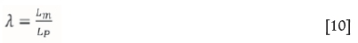
where L_mis the dimension (length) in the model, and L_pthe dimension (length) in the prototype.

To satisfy the geometrical similarity criteria, all dimensions of the prototype must be reduced by λ and all angles in the model must be the same as in the prototype.

Dynamic similarities are concerned with the forces that act on a fluid element. It is necessary that the ratios of the corresponding forces in the model and the prototype be identical for the model to give useful results. Two force ratios are considered when modelling tundish flow patterns: Reynolds number (N_VRe) and Froude number (.%) (Mazumdarand Guthri, 1999). Research by Sahai and Burval (1992) shows that in turbulent regimes such as in the tundish, the magnitude of the Reynolds number, irrespective of geometry or size, is very similar. Therefore Reynold similarities are naturally satisfied as long as the model is operated in a turbulent regime. Following from the above, the only dynamic similarity that should be taken into account when modelling melt flow is the Froude similarity.

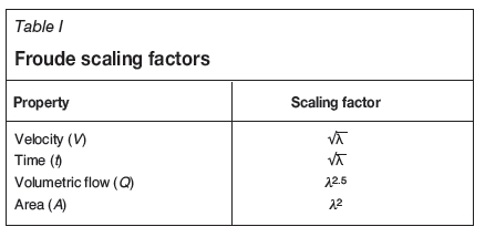
Froude similarity is achieved if Equation [11] is satisfied. From Equation [11], a number of scaling factors for different operating parameter can be formulated in order for the model to remain dynamically similar to the prototype. Table I shows such scale factors.

 

 

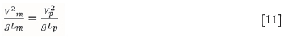
where V_mis the velocity of fluid or inclusion in the model, V_p the velocity of fluid or inclusion in the prototype, g the gravitational acceleration, L_mthe characteristic length of the model, and L_pthe characteristic length of the prototype.

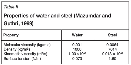
Water is the fluid of choice for modelling the steel phase. This is primarily due to the fact that water at 20°C has a similar kinematic viscosity to that of steel at 1600°C (Mazumdar and Guthri, 1999). Table II shows the properties of water and steel. As can be seen, the kinematic viscosity of steel is 91.3% of the kinematic viscosity of water.

 

 

To simulate the slag layer, a variety of fluids are used, including modified silicon oils, benzene, and paraffin (Chattopadhyay, Isac, and Guthri, 2010, Hsagemann et al., 2013). Krishnapisharody and Irons (2008) recommend the use of paraffin oils for modelling tundish slag when water is used to model the steel melt. A similarity criterion known as the Weber number (We) can be used to evaluate the difference between the modelled system and the prototype tundish with respect to surface tension forces. The Weber number is the ratio of momentum to interfacial tension force, given by Equation [12] (Chattopadhyay, Isac, and Guthri, 2010).

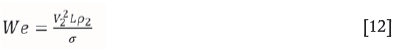
where V₂is the velocity of the melt phase or water phase, L the characteristic length of the tundish, ρ₂ the density of the melt or water phase, and a the interfacial surface tension between steel melt and slag phase.

Ideally, the ratio use of the model Weber number and the prototype Weber number should be unity. By using a combination of Equation [11] and Equation [12], one can calculate the ratio of the Weber number for the two systems in this study.

To maintain both significant geometric and dynamic similarities, not all dimensions can be scaled by λ. To maintain geometric similarity between the bath level of the prototype and that in the model, the outlet cross-sectional area of the model must disobey the similarity criteria or else the model may overflow or drain out. The outlet cross-sectional area in the model is calculated and designed to maintain similarity between the prototype bath level and model bath level. As a consequence:

If the tundish model is operated at steady state, the outlet cross-sectional area of the model can be calculated to satisfy Equation [14]:

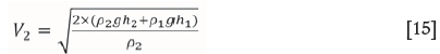
where Q is the volumetric flow of water, A_outm the cross-sectional area of the outlet nozzle in the model, and V₂the velocity of water at the outlet nozzle.

where h₁ is the simulated slag layer thickness and h₂ the simulated melt phase thickness.

Flow characterization in physical models

A flow characterization study is a key starting point when it comes to understanding a reactor or any metallurgical vessel or optimizing its performance. Flow characterization results are the first point of comparison between a numerical model and a physical model.

Typically in such studies, a tracer (salt, dye, or acid) is injected in the inlet stream of the vessel. Its concentration is then monitored at the outlet of the vessel as a function of time. A plot of the tracer concentration at the outlet ports against time is known as the residence time distribution (RTD) curve. The RTD of the vessel can then be analysed to gain knowledge of the flow patterns inside the vessel. Such an analysis involves calculating plug flow volume fraction, dead volume fraction, and mixing volume fractions. Research on tundish flow patterns has shown that tundishes exhibit characteristics of a combined flow model, with dispersed plug flow (Jha, Rao, and Dewan, 2008; Joo and Guthrite, 1991; Tripath and Ajmani, 2005).

For this study, it is worthwhile to physically perform the RTD study for comparison with the numerical determined RTD plot to ensure that the flow patterns are numerically modelled correctly.

Numerical modelling methods

Numerical methods makes use of computer packages to solve a series of fluid mechanics differential equations in 3D or 2D space. Whereas physical modelling incorporated with fluid flow characterization gives quantitative results about what is happening in the vessel, numerical modelling allows the investigator to gain both detailed visual and quantitative information about the flow patterns inside the vessel. In addition to this, numerical simulations allow the investigator to gain knowledge about turbulence, pressure changes, and velocity patterns inside the vessel. Results from numerical models can be verified by comparing them to results from a physical model study. Once verified, the numerical model can be adapted for use in a variety of situations without the need for any experimental work. The numerical modelling in this study was done in ANSYS® Fluent; the numerical modelling theory will thus follow the nomenclature used in this package.

In order to model fluid flow, two main equations must be solved. These are the conservation of mass equation, otherwise known as the continuity equation Equation [16], and the conservation of momentum equation Equation [17] (ANSYS, 2011).

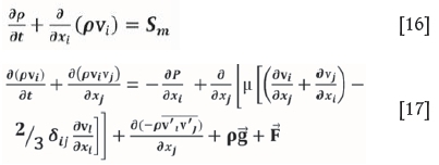
where ρ is the density of the fluid, v_{the velocity component of the fluid in the ijk plane, P the static pressure, μ the molecular viscocity, l the unit tensor, g the gravitational acceleration, and F bodily forces

In Equation [16], the first term relates to change of density with time, the second is change of mass as a result of convection. S_mrelates to source terms in the system, (inputs or outputs, reactions, and evaporation). In Equation [17] the first term represents change of momentum with time, followed by change of momentum due to convection, change of momentum due to pressure changes, change of momentum due to molecular and turbulence shear stress, change of momentum due to Reynolds stresses, change of momentum due to gravitational forces, and lastly change in momentum due to bodily forces (ANSYS, 2011).

To close Equation [17], Reynolds stresses must be known. In particular, the average fluctuating component of the fluid velocity must be known before the velocity flow field is known (Bakker, 2008). A common approach to overcome this is to use the Boussinesq hypothesis, which relates Reynolds stresses to the mean velocity gradient.

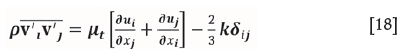
Mathematically this is represented by (ANSYS, 2011):

where μ_tis the turbulent viscocity and k the turbulent kinetic energy.

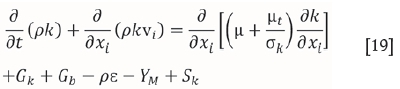
This hypothesis forms the basis of the popular k-ε model, k-ω model, and Spalart-Allmaras model used to resolve turbulence (Bakker, 2008). In the k-ε models (standard and realizable), two extra equations are solved: turbulence kinetic energy (k) and dissipation of turbulence kinetic energy (ε).

Turbulence kinetic energy is calculated from Equation [19]:

while the dissipation of turbulence kinetic energy (ε) can be calculated from:

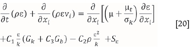
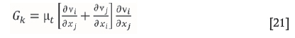
where μ_tis the kinematic turbulent viscosity, μ the molecular viscosity, G_bthe generation of turbulent energy due to buoyancy, Y_Mchanges in dilation (compressible fluids), S_k and S_eare user-defined source terms, and G_kthe rate of generation of kinetic energy per unit mass given by:

The turbulent viscosity can then be calculated by:

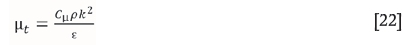
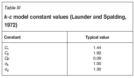
Where C₁, C₂, C₃, a_k, σ _ε , and ϋ _μ are constants. Table III shows the values of these constants. It is important to note that C₃, unlike other constants, is calculated. In the realizable k-ε model the ϋ _μ term is expressed by a differential equation, as opposed to being constant; moreover, the dissipation equation is based on a dynamic equation of the mean-square vorticity fluctuation. This gives the realizable k-ε model an advantage over the standard k-ε model when calculating flows that show strong streamline curvature, vortices, and rotation (Bakker, 2008).

 

 

Two-phase modelling in ANSYS® Fluent can be done by making use of the VOF (Volume of Fluid) model, which tracks the interface on the phases throughout the calculation domain. VOF consists of three methods to model fluid interactions: a methodology to locate the free surface, an algorithm allowing the tracking of free surface as it moves through the computational domain, and a method allowing boundary conditions to be applied at the free surface (Reilly et al., 2013).

In the VOF model a single momentum equation (similar to Equation [17]) is solved for all the phases, where the fluid properties are calculated using Equation [23]. The resulting velocity is shared amongst the phases, i.e. assumed to be equal for all phases present. Interface tracking is achieved by solving a continuity equation which incorporates the volume fraction of each phase, Equation [24] (ANSYS, 2011).

where φ is the average fluid property, such as (density, viscosity, etc.), a_{the volume fraction of the i-th phase, and φ _ι the fluid property of the i-th phase.

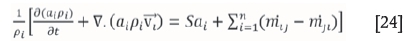
where S_aiis the rate of generation of the i-th phase, and the mass transfer rate of i-th phase into the j-th phase.

For surface tension modelling, one can choose to specify a constant surface tension coefficient or to specify a user-defined equation for surface tension. The VOF model then adds additional tangential stresses that arise due to variable changes in surface tension at the interface. Two surface tension models exist in the VOF model, the continuum surface force (CSF) and the continuum surface stress (CSS). Essentially these models are used to calculate the surface tension force (ANSYS, 2011). In the CSF model the surface tension force is obtained by first calculating the surface curvature from local gradients in the surface normal to the interface. The CSS model is a more conservative model. It avoids calculating the surface curvature to solve for the surface tension force, and thus misses some activity at the interface (ANSYS, 2011).

Boundary conditions

Boundary conditions specify, inter alia, direction of flow, fluid source and sink, and how the flow must behave in certain regions. Boundary conditions can be split into inlet conditions, outlet conditions, wall conditions, and surface conditions.

Inlet conditions involve specifying the position of the inlet, direction of flow, pressure, and whether the velocity has a profile or not. In the case of a turbulent flow entering at the inlet region, the turbulent kinetic energy and dissipation have to be specified. One method of specifying the turbulence at the inlet is to specify the turbulence intensity and hydraulic diameter. The turbulence intensity is given by Equation [25], and the hydraulic diameter is the diameter of the duct (Bakker, 2008):

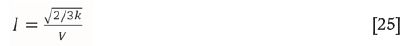
where I is the turbulence intensity, typically 5% for fully developed flow in a pipe, k the turbulence kinetic energy, and V the average velocity in the pipe.

For outlet conditions, the velocity at the outlet is assumed not to have a profile and is given by Equation [15]. Pressure at the outlet is given by the hydrostatic pressure. The outlets are assumed to be open to the atmosphere. All flow property gradients are zero over the outlet region, except for pressure (Bakker, 2008). Wall boundaries are specified to allow the software to know where the boundaries are. The no-slip conditions are used for viscous flows, meaning that the tangential velocity of the fluid closest to the wall has the same velocity as the wall, and that the normal fluid velocity at the wall is zero. The presence of the wall and the choice of no-slip conditions affect how turbulence is dissipated near the wall. In particular, regions closest to the wall are dominated by laminar flow where viscous forces play a significant role. At the outer parts of the wall, momentum transfer is dominated by turbulent conditions. The area between the laminar and turbulent regions is characterized by both laminar and turbulent dissipation of momentum. To resolve flow patterns in near-wall regions, one can use semi-empirical formulae known as wall functions, or modified turbulence models. In the wall functions, the viscosity-dominated region is not resolved, and instead semi-empirical models are used to calculate the flow behaviour in the viscous layer near the wall. In modified turbulence models, the flow behaviour is resolved all the way to the wall. This involves making use of fine mesh sizes near the wall region, which costs in computational time. For ε-based equations, wall-enhanced wall treatment functions are recommended (Bakker, 2008).

For top surface boundary conditions, one can also choose to specify frictionless wall conditions. This has been the norm for most researchers who have worked in the field. They specified the boundary condition at the top of the fluid layer (Cloete, 2014; Kumar, Mazumdar, and Koria, 2008; Mazumdar and Guthri, 1999; Sahai and Emi, 1996; Tripathi and Ajmani, 2011). It is worth mentioning, though, that this boundary condition was used without the presence of a slag phase.

Symmetry conditions are considered when the flow in a vessel is thought to have planes of symmetry. These can be transverse, longitudinal, or vertical. Considering symmetry planes lowers the computational time demand on the software (Bakker, 2008). When this condition is specified, the normal velocity vectors are zero at the symmetry plane, and normal gradients of all variables are zero at the symmetry plane.

 

Physical set-up

Physical modelling set-up

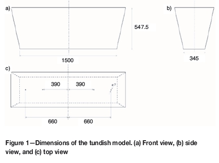
The physical model used in this study was designed by Cloete (2014). The design is based on a tundish used by Kumar, Mazumdar, and Koria (2008), but instead of a scale factor of 1/3 a scale factor of 1/2 was used. The model is constructed from clear 6 mm PVC. It has four strands instead of the normal one or two, and walls inclined at 10°. Figure 1 shows a schematic representative of the tundish. Water was used to model the tundish steel phase, and paraffin to model the slag phase.

 

 

A calculation of the Webber number ratio (We_model/ We_prototype) based on a steel-slag system interfacial surface tension of 1.6 Nm^-1 (Mazumdarand Guthri, 1999; Mills, 2011) and water-to-paraffin interfacial surface tension of 0.048 Nm^-1 (Johansen, 1924) shows that the ratio of the model and prototype Weber numbers is 1.21. This is considered to be close to unity and thus justifies the use of paraffin to model tundish slag.

Table IV lists the dimensions and operating conditions of the prototype (industrial scale) and the model used in this study.

 

 

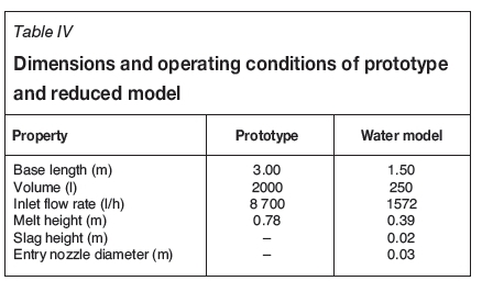
Table V lists the properties of the two liquids used in the water model.

 

 

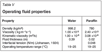
Figure 2 shows a schematic layout of the experimental set-up. Water is fed from the mains to a feed tank, which is kept at a fixed level by a float valve. From the feed tank the water is pumped to the tundish. The inlet flow rate is controlled by a gate valve (V-2) and a rotameter (3). The four ball valves (V-3, V-4, V-5, and V-6) can be closed to stop outlet flow, which is driven by gravity, to allow the tank to fill up. The water from the outlets is fed back to a storage tank (Cloete, 2014).

 

 

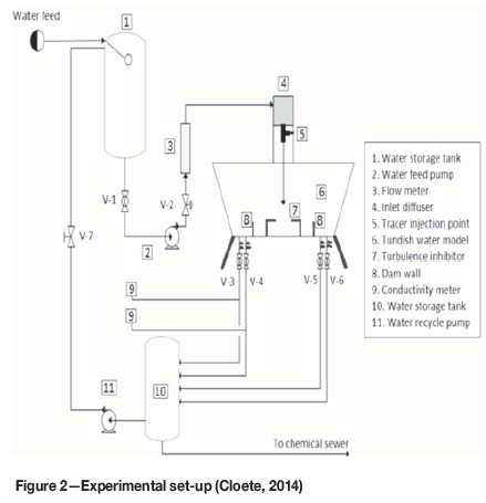
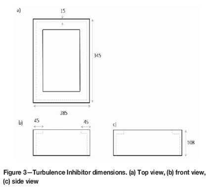
Figure 3 shows the dimensions of the FCD used in this study. The design is based on those used by Cloete (2014) and Kumar, Mazumdar, and Koria, (2008). The FCD was constructed from 15 mm thick grey PVC. It was fixed in position and sealed with silicone.

 

 

Sampling of entrained slag entrainment was done by taking 50 ml samples with a pipette from the tundish while in operation, weighing the sample using a two-decimal-place scale, then calculating the sample's density and then the volume fraction of entrained paraffin at that location using Equation [26]. The densities of water and paraffin used in Equation [26] were determined by taking ten 50 ml samples of each fluid and weighing them. This was done every day during the sampling period to account for changes in water density due to the weather.

 

 

To avoid systematic errors, the location at which a sample was to be taken was programmed into Microsoft Excel® to be random. Five repeats of each sampling location were taken.

To determine where samples were to be taken, Cloete's results were used. Cloete (2014) studied the flow patterns in the tundish model used in this study, and investigated the effect of different FCDs on the melt flow behaviour. However, like other authors, he did not include the slag layer. Based on his work, areas where entrainment at the interface might occur can be predicted. Moreover, dead volumes where entrained 'slag' might accumulate can be identified. This was the basis for the physical grid design and sampling locations. Based on Cloete's results it was decided to sample at a depth of 220 mm (total depth).

Five repeats of each sampling point were taken over a period of 5 hours. The five repeats were averaged to give one value for the volume fraction of entrained paraffin. It is worth mentioning that the residence time of the cold model is 8 minutes, and that the sampling method followed in this study mimicked a number of hits, i.e. a number of ladles transferring melt to the tundish.

Weather changes had a significant effect on the water density, thus sampling had to be done during settled weather conditions. In this study sampling was done over a week to account for weather changes, and each day the density of water was calculated by weighing 50 ml of water and paraffin.

Five repeats of the RTD study were done. The following guidelines applied. When the system had stabilized (after 45 minutes), the tracer was injected into the model via the tracer injection point (see Figure 2). 60 ml of 300 g/l table salt solution was used for these tests. The injection was done over 5 seconds. After injection, the concentration of the tracer in the outlet stream of two strands was monitored using a calibrated conductivity meter. The concentration of the tracer at the outlets was recorded at 30-second intervals for 20 minutes; this is more than twice the theoretical residence time of the model.

Numerical modelling set-up

The realizable k-ε model was used for the turbulence model, while the VOF model was used to model the two faces (water and paraffin).

Boundary conditions

► The velocity inlet was at the top of the entry nozzle. The velocity was specified as 0.614 m/s. The turbulence intensity was left as 5 % and the hydraulic diameter was specified as 30 mm

► On the strand outlets, the settings were left as pressure-based. The default gauge pressure of zero and the turbulence intensity of 5% were used. The hydraulic diameter was specified as 7 mm

► Symmetry conditions were applied along the transverse and longitudinal planes of the tundish, thus reducing the computational domain to a quarter of the full-scale model

► The sidewalls, bottom of the tundish, and FCD walls were specified as no-slip conditions

► No extra boundary conditions were specified at the interface since the continuity equation and momentum equations were naturally satisfied across the interface. The VOF also inherently specifies a balance of forces due to pressure difference across the interface and interfacial tension at the interface.

Solver settings

► The pressure-based solver was used. SIMPLE scheme was used for pressure-velocity calculations

► All convective parameters were first interpolated using first-order upwind, and later changed to second-order upwind once the solutions had stabilized

► Volume fraction was solved using second-order upwind throughout

► Gradients of solutions were evaluated using the least square cell-based scheme. This was chosen to reduce false (numerical) diffusion

► The pressure was interpolated using the PRESTO! scheme.

Flow characterization in numerical modelling

A comparison between the results of a numerical RTD and those of the physical model is often the first step towards validating the numerical results. To study the RTD of a vessel numerically using ANSYS® Fluent, Equation [27] is solved for the tracer element.

where Y_{is the mass fraction of the tracer in the calculation domain, J the effective mass transfer in the calculation domain given by Equation [28], R_{the rate of production of the tracer by reaction, S_ithe rate of production of the tracer via addition, and ρ the density of the primary fluid or fluid in which the tracer is flowing .

where D_iis the molecular diffusion of tracer in the main fluid, Sc_tthe turbulent Schmidt number, with a value of 0.7, and μ_t the turbulent viscosity.

 

Physical modelling observations and results

Observations

While running the physical model, it was noticed that there seemed to be little to no movement of the water-paraffin interface, which implies that there is no turbulence at the interface and that slag entrainment does not take place via turbulence at the interface. There was no visual evidence of paraffin entrainment as a result of shearing at the interface, as was seen by other workers. Small droplets of entrained paraffin (approximately 1 mm) could be seen floating in low concentrations at a depth of 300 mm. Initial measurements showed that a small amount of paraffin is entrained, with a maximum volume fraction of approximately 0.02, even at a depth of 220 mm. These observations suggest that the entrainment of the paraffin 'slag' does not take place via macroscopic shearing of the interface, but by microscopic entrainment, possibly assisted by mass transfer at the steel-slag interface. By studying the interfacial velocities using the numerical model developed in this study, more insight will be gathered on this.

It was also noted that as the pipette was being immersed in the paraffin layer and bulk water phase for sampling, a small amount of paraffin (simulated slag layer) and a mix of 'entrained' paraffin and water from shallower depths (<220 mm) in the bulk water phase tended to be forced into the pipette before a sample could be taken. This caused a high bias in the results. The bias resulting from the pipette going through the paraffin phase can be measured by sampling the model at 220 mm depth when there is no flow, i.e. paraffin phase and water phase present, close all the strand outlets, and sample at 220 mm depth with no flow entering the model. Thus this error can be eliminated. The error or bias resulting from the 'entrained' paraffin and water mixture could not be measured. See the comparison between the numerical and physical model results for how much this error affected the results.

Entrained slag behaviour

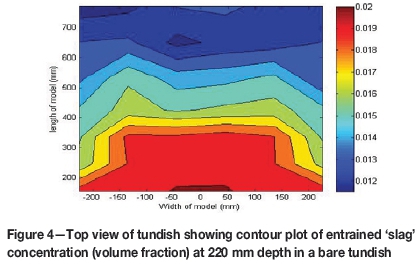
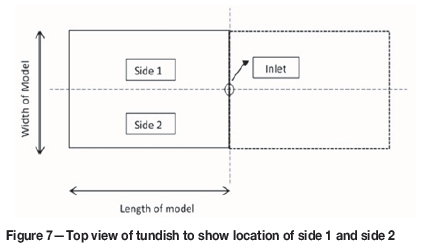
Figures 4 and Figure 5 show contour plots of entrained paraffin (slag) in a bare tundish and a tundish with FCD respectively. The zero on the x-axis represents the centreline where the inlet is located. The y-axis represents the length of the model. Note that 130 mm of sampling location was lost due to structural interference, hence the y-axis starts at 200 mm.

 

 

 

 

 

 

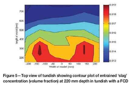
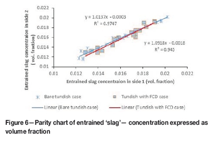
To investigate the use of symmetry conditions along the longitudinal and transverse centrelines in the numerical model, a parity chart based on entrained 'slag' concentrations was drawn, shown in Figure 6. Figures 4 to 6 should be examined in conjunction with Figure 7 for orientation and an explanation of the meaning of side 1 and side 2.

 

 

From Figure 4 it can be seen that entrained slag in a bare tundish tends to accumulate in the region closest to the inlet. The concentration of entrained slag tends to decrease towards the endwalls. This is a similar to findings of Solhed, Jonsson, and Jönsson (2008). Interestingly, a slightly similar pattern is seen in the tundish with a flow control device (Figure 5); however, with the FCD device the entrained 'slag' seems to appear in more localized pockets that form two parallel slits. From the parity charts (Figure 6), it can be seen that the concentration of entrained 'slag' is indeed symmetrical about the longitudinal centreline. These results make it acceptable to numerically model only a quarter of the tundish and assume symmetry planes along the longitudinal and transverse centrelines, instead of the full tundish. This saves a significant amount of computational time when solving the flow equations.

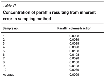
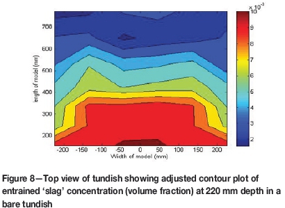
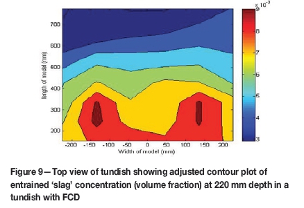
As noted, when the pipette was being immersed in the paraffin layer and bulk water phase for sampling, a small amount of paraffin (from the simulated slag layer) and a mix of 'entrained' paraffin and water from shallower depths (<220 mm) in the bulk water phase tended to be forced into the pipette, due to hydrostatic pressure, before a sample could be taken. This caused a high bias in the results shown in Figure 4 and Figure 5. To account for this bias, ten blank samples (at 220 mm depth with no flow) were taken and the concentration of paraffin was measured. Table VI shows the results from this test. Since this error is inherent throughout the model it can be subtracted from the data shown in Figure 4 and Figure 5, thus giving more accurate results. Figure 8 and Figure 9 show results with reduced inherent error. It is important to note that although further analysis will be done using these figures (Figure 8 and Figure 9), these results still contain a portion of the inherent sampling error and thus could be higher than the true concentration of the entrained paraffin. However, of importance to this study is the ability of the numerical model to predict the entrained slag behaviour and to give the same order of magnitude of entrained paraffin concentration as in the physical model, as opposed to the actual value entrained paraffin concentration.

 

 

 

 

 

 

Numerical modelling results

Numerically predicted RTD

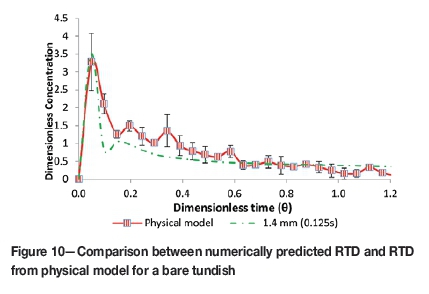
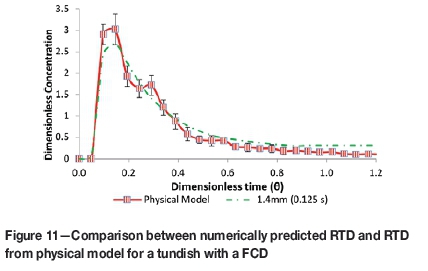
Figures 10 and 11 show a comparison between the numerically predicted RTD and the physically produced RTD curve for the bare tundish and tundish with FCD, respectively. In both cases (the bare tundish and tundish with FCD) a match between the physical model and the numerical model was achieved with a mesh of 1.4 mm at a time step of 0.125 seconds. It is quite interesting to note that the spread was numerically modelled well in the FCD case, but the details of the second peak were not. In the bare tundish, the spread was not modelled well but the details of the second peak were captured well. This allows for further analysis of the numerical model.

 

 

 

 

Numerically predicted entrained slag behaviour

Figures 12 and 13 show numerically developed contour plots of entrained paraffin concentration (slag) at a depth of 220 mm in a bare tundish and a tundish furnished with a FCD respectively. As in the physical model, the entrained slag concentration is highest behind the inlet shroud. The concentration of entrained slag tends to decrease towards the endwalls. It is interesting to note that the concentration of entrained slag is lower in the case of the FCD than in the case of the bare tundish (38% lower, based on the highest entrained 'slag' concentration). However, this does not imply that less slag is entrained in the case of the FCD. Such a conclusion can be made only if the concentration of the entrained 'slag' were to be measured at the strands for both cases. This was not done in this study due to the complexity of acquiring accurate results, given the low concentration. It is also interesting to note that the numerically predicted entrained slag concentration is 55% and 68% lower than found in the cold model for the bare tundish and tundish with FCD respectively (based on highest seen concentration).

 

 

 

 

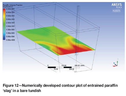
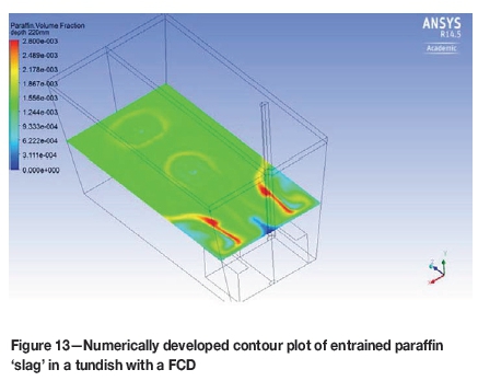
This high bias in the cold model results was noted in the observations. It results from fluid in shallower depths being pushed into the pipette as a result of hydrostatic pressure. It is important to note that an attempt was made to reduce this error and the residual error as highlighted earlier.

Flow patterns that lead to slag entrainment

Having found a numerical model that can predict the slag entrainment behaviour and flow patterns, the mechanism that results in tundish slag entrainment can be studied using the numerical models.

Bare tundish flow patterns

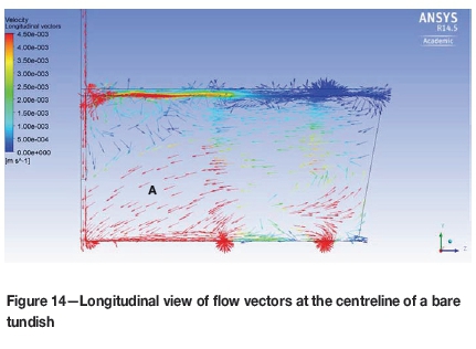
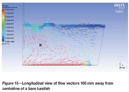
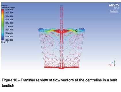
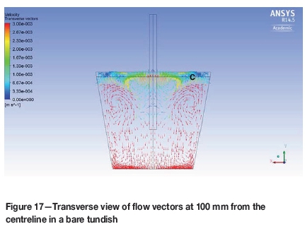
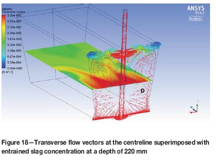
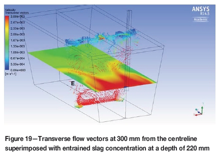
Figures 14 and 15 depict the longitudinal view of the flow patterns in a bare tundish. In Figure 14 it can be seen that the flow exits the inlet shroud, impinges at the bottom of the tundish, and reports to the inner strand. The displacement of the melt at the bottom of the tundish causes a draft of melt from the outer walls of the tundish (region A). In this view it can be seen that there is no excessive tangential flow close to the steel-slag interface. Thus the entrainment does not arise from longitudinally directed flow. In Figure 15, downwards-directed flow from the sidewalls can be seen (region B). Figure Figures 16 and 17 depict the flow patterns in transverse view. The flow impinges at the bottom of the tundish, and then moves up the sidewalls to cause shearing below the steel-slag interface (region C). It is this flow being assisted by mass transfer at the interface that is believed to aid slag entrainment in bare tundishes. Figure 18 and 19 show the flow patterns in the transverse plane superimposed on a contour plot of entrained paraffin 'slag' concentration at a depth of 220 mm. It can be seen that the areas of high paraffin (slag) concentration are the areas where the flow that impinged on the bottom of the tundish falls on itself (region D). The entrained slag is then carried down by the flow until the flow turns into itself in region D. As the flow that rises up the sidewalls decreases, less slag is seen in the steel phase in region E (see Figure Figure 19).

 

 

 

 

 

 

 

 

 

 

 

 

Tundish with FCD flow patterns

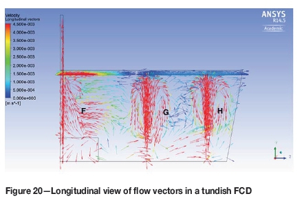
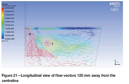
Figure Figures 20 and 21 show longitudinal flow patterns in a tundish with a FCD. The flow exits the inlet shroud and is immediately directed to the steel-slag interface by the FCD, as intended (region F). There are two clear vortices above the inner and outer strand, which did not show in previous studies such as that by Cloete (2014). These vortices do not extend to the top of the slag layer, possibly due to the viscosity of the paraffin (slag) layer (regions G and H). Similarly to the bare tundish case, the displacement of fluid close to the inlet region causes flow to the inlet region from nearby areas (region I).

 

 

 

 

The transverse view (Figure Figure 22) shows that most of the flow exiting from the inlet shroud is reflected from the bottom of the tundish and directed to the slag layer, as intended. This flow then impinges on the slag layer, where it results in tangential flow to the slag layer (region J). This tangential flow can even be seen in. It is quite interesting to note that a similar tangential flow in the bare tundish is created by the FCD, the only difference being that in the FCD case, the flow is from inside going out to the sidewalls, whereas in the bare tundish case it is from the sidewalls going towards the inlet region. It is possible that the entrainment first takes place in region J, where the flow is tangential to the interface.

 

 

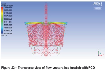
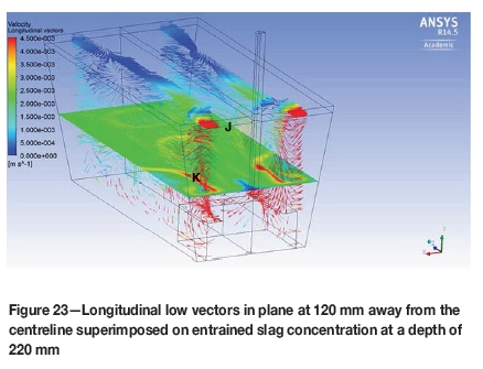
Figure Figure 23 shows flow patterns in the longitudinal plane 120 mm away from the centreline superimposed on the entrained 'slag' concentration at a depth of 220 mm. From this figure it is evident that the entrained 'slag' from area J moves with the prevailing flow to accumulate in region K.

 

 

Slag entrainment mechanisms in a bare tundish

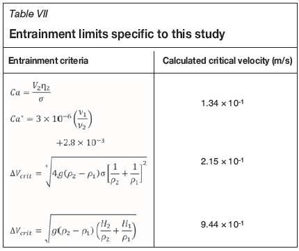
In order to understand the main mechanism behind slag entrainment in tundishes, it is important to understand the critical velocities at which slag entrainment takes place and then compare these to the numerically simulated interfacial velocities to identify which mechanisms are responsible for slag entrainment. Table VII shows the various slag entrainment mechanisms considered in this study, the criteria for entrainment, and the calculated critical velocities for the water-paraffin case used in this study. It can be seen that the critical velocities for slag entrainment in the water model range from 1.34 χ 10^-1 to 9.44 χ 10^-1 m/s.

 

 

Figures 24 to 26 show velocity vectors tangential to the water-paraffin interface (steel-slag interface) in the bare tundish case. In Figure 25 it can be seen that there are no clear tangential velocities even at 10 mm below the interface. However, in Figure 26 one can see relatively high velocity vectors tangential to the interface. The highest of these vectors is 3 χ 10^-3 m/s. However, this is significantly lower than the velocities calculated for macroscopic shearing methods considered in Table VII.

 

 

 

 

 

 

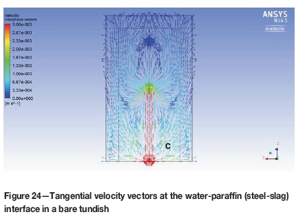
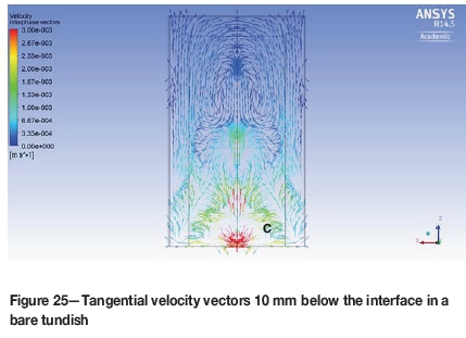
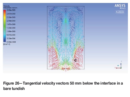
The lack of tangential velocities directly at the interface suggests that the paraffin initially moved by mass transfer across the interface, and that shearing occurs only at a depth of 50 mm.

Slag entrainment mechanisms in a tundish with FCD

Figures 27-29 depict tangential velocity vectors to the interface at varying depths in a tundish with FCD. It can be seen that even at just below the interface, high tangential velocities exist (the highest is 6 χ 10^-3 m/s). However, none of these velocity vectors pass the threshold of 1.34 χ 10^-1 m/s.

 

 

 

 

 

 

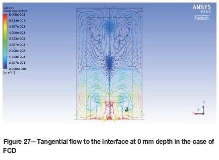
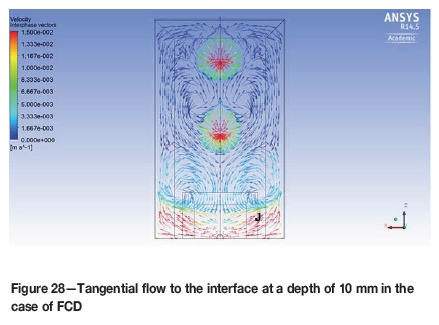
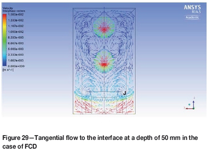
This provides proof that entrainment in a tundish with a FCD does not take place via the macroscopic methods considered in this study, but perhaps takes place via mass transfer across the interface, assisted by minor velocity shearing close to the interface.

 

Conclusions

Tundish slag behaviour

Results from the physical model showed that the steel-slag interface remains immobile during operation with both the bare tundish and the tundish with a FCD. Sampling of entrained paraffin 'slag' at a depth of 220 mm showed that the entrained tundish 'slag', in the case of both bare and FCD tundishes, tended to concentrate behind the inlet shroud. There is less concentration of entrained slag towards the tundish endwalls.

Numerical model for slag entrainment

A numerical model was developed using the realizable k-model with mesh size of 1.4 mm and a time step of 0.125 seconds. The numerically modelled residence time distru-bution and entrained slag behaviour agreed strongly with those of the physical model.

Mechanisms for tundish slag entrainment

An analysis of numerically developed tangential velocities below the steel-slag interface (0-50 mm below the interface) showed that in both the bare tundish and tundish with a FCD, the tangential velocities are a factor of 10 less than the critical velocities necessary for Kelvin-Helmholtz instability and any other form of macroscopic entrainment.

The existence of relatively high tangential velocity vectors only 10 mm or more below the steel-slag interface, resulting in shearing of the slag layer, suggests that the slag moves across the interface by mass transfer. Then, shearing caused by low tangential velocities below the interface is responsible for carrying the slag into the bulk steel phase.

It can therefore be concluded that slag entrainment in both the bare tundish and the tundish with a FCD takes place by two mechanisms: mass transfer across the interface and low-velocity shearing.

 

Recommendations

Incorporate the slag phase in future tundish studies

This study has resulted in new information being added to the already extensive literature on tundish operations. It was shown that a physical model and a numerical study involving tundish slag can be constructed with relative ease.

To provide more complete models, it is recommended that future work involving tundishes includes the slag layer. This will help provide more comprehensive solutions that will aid in improving tundish performance.

Validate both numerical and physical data with experimental work

Although appropriate dimensionless numbers were used in this work, and the results ought therefore to be the same as the prototype results, it is still recommended that the concentration of slag entrained at the depths studied in this work and the mechanism of tundish slag entrainment be verified in an industrial tundish.

Incorporate inclusion modelling (numerical and physical)

In this study the concept of tundish modelling has been expanded by including a slag phase. However, there is still scope to extend studies by incorporating inclusion modelling in the existing tundish slag model. Such work will help researchers to gain a complete understanding of how the tundish behaves under the influence of a flow control device. The size and properties of the particles to be used will have to satisfy the requirements of dimensionless number similarities.

 

References

ANSYS. 2011. ANSYS Fluent theory guide, version 14.         [ Links ]

Bakker, A. 2008. Computational Fluid Dyanamics. http://www.bakker.org/ [Accessed 27 April 2014].         [ Links ]

Chattopadhyay, K., Isac, M., and Guthri, R.I.L. 2010. Physical and mathematical modelling of steelmaking tundish operations: a review of the last decade (1999-2009). ISIJ International. vol. 50, no. 3. pp. 331-348.         [ Links ]

CLOETE, J.H. 2014. Flow analysis of a four-strand steelmaking tundish using physical and numerical modelling. Master's thesis, University of Stellenbosch.         [ Links ]

Feldbauer, S. and Cramb, A.W. 1995. Proceedings of the 13th Process Technology Conference, Nashville, TN, 2-5 April 1995. Iron and Steel Society, Warrendale, PA. pp. 327-340.         [ Links ]

Hagemann, R., Rüdiger, S., Heller, H.P., and Scheller, P.R. 2013. Model investigations on the stability of the steel-slag interface in continuous- casting process. Metallurgical and Materials Transactions, vol. 44, no. 1. pp. 80-90.         [ Links ]

Harman, J.M. and Cramb, A.W. 1996. A study on the effect of fluid physical properties on droplet emulsification. Proceedings of the 79 th Steelmaking Conference, Pittsburgh, PA, 24-27 March 1996. Iron and Steel Society of AIME, Warrendale, PA. pp. 773-784.         [ Links ]

Hibbeler, L.C. and Thomas, B.G. 2010. Investigation of mold flux entrainment in CC molds due to shear layer instability. Proceedings of the 2010 AISTech Steelmaking Conference. Association for Iron & Steel Technology, Warrendale, PA. pp. 1215-1230.         [ Links ]

Iguchi, M., Yoshida, J., Shimizu, T., and Mizuno, Y. 2000. Model study on entrapment of mold powder into molten steel. ISIJ International, vol. 40, no. 7. pp. 658-691.         [ Links ]

Jha, P.K., Dash, S.K., and Kumar, S. 2001. Fluid flow and mixing in a six strand billet caster tundish: a parametric study. ISIJ International, vol. 41, no. 12. pp. 1437-1446.         [ Links ]

Jha, P.K., Rao, P.S., and Dewan, A. 2008. Effect of height and position of dams on inclusion removal in a six strand tundish. ISIJ International, vol. 48, no. 2. pp. 154-160.         [ Links ]

Johansen, E.M. 1924. The interfacial tension between petroleum products and water. Industrial and Engineering Chemistry, vol. 16, no. 2. pp. 132-135.         [ Links ]

Joo, S. and Guthrite, R.I.L. 1991. Heat flow and inclusion behaviour in a tundish for slab casting. Canadian Metallurgical Quarterly, vol. 30. pp. 261-269.         [ Links ]

Krishnapisharody, K. and Irons, G.A. 2008. An extended model for slag eye size in ladle metallurgy. ISIJ International, vol. 48, no. 12. pp. 1807-1809.         [ Links ]

Kumar, A., Koria, S.C., and Mazumdar, D. 2007. Basis for systematic hydrodynamic analysis of a multi-strand tundish. ISIJ International, vol. 47, no. 11. pp. 1618-1624.         [ Links ]

Kumar, A., Mazumdar, D., and Koria, S.C. 2008. Modeling of fluid flow and residence time distribution in a four-strand tundish for enhancing inclusion removal. ISIJ International, vol. 48. pp. 38-47.         [ Links ]

Launder, B.E. and Spalding, D.B. (eds.). 1972. Lectures in Mathematical Models of Turbulence. Academic Press, London.         [ Links ]

Mazumdar, D. and Guthri, R.I.L. 1999. The physical and mathematical tundish systems. ISIJ International, vol. 39, no. 6. pp. 524-547.         [ Links ]

Mills , K. 2011. The estimation of slag properties. Proceedings of Southern African Pyrometallurgy 2011, Misty Hills Conference Centre, Muldersdrift, Gauteng, South Africa, 6-9 March 2011. Jones. R.T. and den Hoed, P. (eds.). Southern African Institute of Mining and Metallurgy, Johannesburg, pp. 1-52.         [ Links ]

Milne-Thomson, L.M. 1968. Theoretical Hydrodyanamics. 5th edn. Macmillan, London.         [ Links ]

Nagaoka, T., Radot, J.P., Reynolds, T., Vaterlaus, A., and Wolf, M. 1986. The basic concept of the extra low head caster for slabs and blooms. Proceedings of the 69th Steelmaking Conference, Washinton, 6-9 April 1986. Lucenti, G.S. (ed.). Iron and Steel Society of AIME, Warrendale, PA. vol. 69. pp. 799-810.         [ Links ]

Reilly, C., Green, N.R., Jolly, M.R., and Gebelin, J. 2013. The modelling of oxide film entrainment in casting systems using computational modelling. Applied Mathematical Modelling, vol. 37. pp. 8451-8466.         [ Links ]

Sahai, Y. and Burval, M.D. 1992. Proceedings of the 50th Electric Furnace Conference, Atlanta, GA, 10-13 November 1992. Iron and Steel Society of AIME, Warrendale, PA. pp. 469-474.         [ Links ]

Sahai, Y. and Emi, T. 1996. Melt flow characterization in continuous casting tundishes. ISIJ International, vol. 36, no. 6. pp. 667-672.         [ Links ]

Sahai, Y. and Emi, T. 2008. Tundish Technology for Clean Steel Production. World Scientific Publishing, Singapore.         [ Links ]

Senguttuvan, A. and Irons, G.A. 2013. Model studies on slag metal entrainment in gas-stirred ladles. AIST Transactions, vol. 1, no. 1. pp. 230.         [ Links ]

Solhed, H. and Jonsson, L. 2003. An investigation of slag floatation and entrapment in a continuous-casting tundish using fluid-flow simulations, sampling and physical metallurgy. Scandinavian Journal of Metallurgy, vol. 32, no. 1. pp.15-30.         [ Links ]

Solhed, H., Jonsson, L., and Jönsson, P. 2008. Modelling of steel/slag interface in a continuous casting tundish. Steel Research International, vol. 79, no. 5. pp. 348-357.         [ Links ]

Tripathi, A. and Ajmani, 2005. S.K. Numerical investigation of fluid flow phenomenon in a curved shape tundish of billet caster. ISIJ International, vol. 45, no. 11. pp. 1616-1625.         [ Links ]

Tripathi, A. and Ajmani, S.K. 2011. Effect of shape and flow control devices on the fluid flow characteristics in three different industrial six strand billet caster tundish. ISIJ International, vol. 51, no. 10. pp. 1647-1656.         [ Links ]

 

 

Paper received Aug. 2016
Revised paper received Nov. 2016