GENERAL PAPERS

 

Financial analysis of the impact of increasing mining rate in underground mining, using simulation and mixed integer programming

 

 

A. Salama^I; M. Nehring^II; J. Greberg^I

^IDivision of Mining and Rock Engineering, Department of Civil, Mining and Environmental Engineering, Lulea University of Technology, Lulea, Sweden
^IISchool of Mechanical and Mining Engineering, The University of Queensland, St Lucia, QLD, Australia

 

 

---

SYNOPSIS

This paper challenges the traditional notion that mine planners need to plan production so as to incur the lowest mining cost. For a given mine configuration, a mine that increases its mining rate will incur increased mining costs. In an environment in which operations are fixated on cost reduction, a proposal that increases costs will not be readily accepted. Such a proposal requires financial justification-the increase in costs might be recuperated by the additional production. This paper evaluates the net present value (NPV) across a range of copper prices for two underground orebodies located at different depths, using a production rate of 300 kt per quarter and a scenario that introduces additional equipment and costs for 450 kt per quarter. The evaluation was based on the changes of NPV for the orebody located at a shallow depth compared with the orebody at a greater depth. Discrete event simulation combined with mixed integer programming was used for analysis. Unlike traditional sensitivity analysis, this study re-optimizes the mine plan for each commodity price at each production rate. The results show that, for the low mining rate at the final copper price, an NPV of A$1530.64 million is achieved, whereas an NPV of A$1537.59 million is achieved at a higher mining rate. Even though pushing mining rates beyond traditional limits may increase mining costs, this option may be beneficial at certain commodity prices, particularly when prices are elevated.

Keywords: mining rates, commodity price, simulation, mixed integer programming.

---

 

 

Introduction

A traditional notion among mine planners is that mining rates should be planned in such a way as to reduce production costs. This concept generally relates to the mining rate that results in the highest machine utilization for the selected equipment. Although an existing mine may consider increasing its mining rate by adding equipment to a given mine configuration, this typically increases mining costs. In an environment in which operations are fixated on cost reduction, a proposal to increase costs may be very difficult to argue for. The value of the mine plan is well recognized as varying with the mining rate for a given orebody (Smith, 1997).

The mining rate is usually not constant for the life of an operation, and the decision to increase or decrease the rate depends on many factors, including market conditions and the size of the resource. Research focusing on determining the optimal mine plan and, simultaneously, allowing a variable mining rate and a varying commodity price over the life of the operation, is distinctly lacking.

Most mine planning adopts a traditional single rate at a fixed commodity price. Brennan and Schwartz (1985) developed a mine plan using variations in the metal price without changing the mining rate. The authors proposed that a mine can continue its operations only if the metal price is high enough to maintain a positive cash flow. Yearn (1992) and Baqun (2001) developed methods to determine the optimal cut-off grade and mining rate to yield the maximum net present value (NPV). In both cases, the metal price was fixed for the life of the deposit and little discussion ensued on the degree to which the system will change considering metal price variations. King (2000) developed a mine plan model with dynamic programming using Lane's cutoff grade theory for a fixed mining rate. An approach was later developed to allow variable mining rates at a fixed price in the value optimization of the mine plan. Mclsaac (2008) employed golden search optimization using simulation-based models that consider metal price uncertainty to determine a robust fixed cut-off grade. However, his evaluation showed that the mining rate was fixed for the entire life of the underground mining operation. Salama, Nehring, and Greberg (2014) presented an optimization of the value of the mine plan across a range of metal prices without considering a variable mining rate. They suggest that when mining operations seek to gain as much value as possible, continuing to operate under the same mine plan is inappropriate if commodity prices change during the course of operation. In addition, they suggest that a mining rate that can be altered during the life of the mine by reconfiguring the number of pieces of equipment, even if mining costs increase, should be explored as a means to further maximize the value of the mine plan.

Much of the literature shows the validity in generating new mine plans when commodity prices change under fixed mining rate conditions and the same general equipment configuration. The aim of this paper is to investigate the validity of mine plan value maximization across ten copper price scenarios from A$5250 per ton Cu to A$9750 per ton, in A$500 per ton increments, while allowing a variable mining rate from 300 kt to 450 kt per quarter during the life of an underground sublevel stoping copper operation. The analysis was performed using discrete event simulation combined with mixed integer programming. Simulation was first used to compute the appropriate mining costs at the current and increased mining rates for the operation. Mixed integer programming (MIP) was then used to generate optimal schedules and mine plans for the selected range of copper prices. Unlike a traditional sensitivity analysis, this study re-optimizes the mine plan for each commodity price at each mining rate. An explicit value in each case is attributed to the value resulting from a change in commodity price, and more importantly, the value resulting from an optimization of the mine plan.

 

Mining rate

The mining rate selected significantly influences the optimization process. The selection may be based on an empirical formula or economic measures (Tatman, 2001). Taylor (1986) produced an equation to estimate the mining rate on the basis of the size of the deposit, known as Taylor's Rule, which is still used today. However Taylor's Rule has limitations regarding several factors, such as hoisting capacity, mine depth, and geometry of the deposit. Tatman (2001) developed an empirical equation for steeply dipping underground deposits by taking into account the geometry, rather than the size, of the orebody. Economic measures such as NPV should ultimately have a large weighting when considering one mining rate over another. NPV is the summation of all discounted future cash flows over the life of the operation. Smith (1997) discussed the economic characteristics affecting the selection of the optimum mining rate from an investor's point of view. He suggested that the mining rate can be selected by maximizing the NPV and discounted cash flow return on investment. Once the mining rate is determined and the operations start, it is difficult, and often capital-intensive, to change the mining rate to a significant extent (Ding, 2001). An expansion of mining capacity may occur for several reasons, such as new geological information and economic changes. In the early stage, the mining rate is defined on the basis of the orebody delineated from very limited geological information and all materials inside the orebody are assumed to be accessible. At a later stage, the grade distribution within the orebody may change the production sequence because some of the material considered as waste may become mineable if extracted with adjacent high-grade material. For example, if the price of the contained mineral falls, part of the reserve may become unprofitable to mine. If the price exceeds that which was initially used, then production should be modified to reflect the new economic circumstances (Hall and Stewart, 2004). For existing operations that have a flexible hauling system, the mining rate can be increased by adding more equipment, although doing so decreases the equipment utilization. An increase in equipment tends to result in higher mining costs.

Equipment productivity is very important when planning and designing a mining operation. Some of the factors that affect equipment productivity include the mine schedule, number of cycles per hour, location of dig and dump sites (travel time), operator proficiency, digging conditions, and bucket capacity (Barabady and Kumar, 2008). The mine design and layout is heavily influenced by the equipment used to carry out the extraction, and the final equipment selection can be made only after completion of the mine configuration. The mine planning team always selects equipment and designs the mine in such a way as to maximize equipment utilization (Topuz and Baral, 1988). This process includes, but is not limited to, designing pushback widths (in the case of an open pit) or the size and location of underground drives (in the case of underground operations) to be large enough to allow easy loading and haulage without excessive interaction with other equipment. This study investigates whether an increase in mining rates by employing more equipment, which results in an increase in mining cost, is an appropriate strategy under existing mine configurations at different commodity price scenarios.

 

Simulation and mixed integer programming

The study was performed using a combined iterative approach with discrete event simulation and mixed integer programming. Discrete event simulation is the modelling of stochastic dynamic systems in which the variables change only at discrete points in time, making it very applicable for modelling complex systems such as, for instance, mining operations. Lately, the use of discrete event simulation for mining studies has increased, and has shown wide applicability to various operations, both underground and open-pit (Govinda, Vardhan, and Rao, 2009). For instance, the method has been used for fleet optimization in underground mining, comparison of timing and efficiency between drills, mine to mill production systems, and maintenance scheduling (Banks et al., 2010). A number of simulation software packages are available on the market, such as GPSS/H, AutoMod, and SLAM. In this analysis, the General Purpose Simulation System/Henrikson (GPSS/H) was used. The operational cycles from the working faces at which LHDs load material and dump it into orepasses was modelled. The simulation showed the number of LHD machines required to haul 450 kt of ore to each respective orepass. The simulation results were further used to compute the associated mining costs. Mixed integer programming (MIP) was then used on the basis of the results from the discrete event simulation model to generate optimal schedules and mine plans for the selected range of copper prices. Discrete event simulation combined with MIP has been successfully used in prior studies that proved the benefits of combining the two tools (Salama, Nehring, and Greberg, 2014).

Arguably, MIP is the most common optimization technique used to solve highly complex and constrained problems in the mining industry. MIP combines linear programming (LP) with the additional constraint that some variables must take on an integer value. This integer variable is typically represented as a binary '1' or '0' value to reflect a 'yes' or 'no' decision (Winston and Goldberg, 2004). Reverting from LP to MIP in the mining context is most common when assigning equipment and resources to various operations within the mine is necessary. These resources can only be allocated in their entirety and, as such, the decision whether or not to allocate the full resource across a number of working areas must be made. Similar to LP, the constraints in MIP form a multi-dimensional volume encompassed by linear functions. A number of solution processes, including the simplex method, the branch and bound method, and cutting planes, are generally built into commercially available solvers to extract the optimal solution from this multi-dimensional volume (Floudas, 1995). MIP models have been generated and extensively used to successfully solve a number of mining-related problems by Trout (1995), Topal (2008), Nehring, Topal, and Little (2010), Yap et al., (2013), and Salama, Nehring, and Greberg (2014).

 

Case study

A case study on an underground orebody amenable to sublevel stoping was used to investigate the change in NPV attributed to a new mine plan at a variable commodity prices and mining rates. Whereas some of the data for this particular case study was conceptual in nature, it is based on real operational scenarios with stope tonnages, grades, resource limitations, and sequencing interactions reflective of a real sublevel stoping operation. The setting of this mine was a typical remote mining region in Australia. As such, all figures are quoted in Australian dollars (A$). The value attributed to each stope was based on the operating cash flows generated. The cash flows were obtained by subtracting the revenues from the operating costs under each scenario. The operation investigated extracts copper-bearing ore from a deep underground mine that exploits two copper-bearing orebodies striking east-west and dipping at 70-75 degrees in a southerly direction.

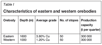
The sublevel stoping production was modelled according to four phases-internal development, followed by production drilling (three months), extraction (three months), and backfilling and consolidation (three months)-which takes each stope nine months to complete. Overall Mineral Reserves were calculated at 15 Mt at an average grade of 2.50% Cu for 375 kt of copper metal. The steady-state production rate for this operation was 450 kt per quarter (1.8 Mt/a). At these production rates, this operation is expected to have a mine life of at least 8.5 years, or 34 quarters. The production capacity for each orebody was 300 kt per quarter. Production scheduling incorporates all stopes from both orebodies to generate a life-of-mine plan at quarterly intervals. Therefore, this process requires both orebodies to be in production in each scheduling period to achieve the overall mining rate of 450 kt. Table I shows some of the parameters for the eastern and western orebodies being mined. Each stope had a size of 25x25x100 m to maintain geotechnical stability. The western orebody was considered low grade and the eastern orebody was considered high grade.

 

 

Stoping conditions at this depth within the western orebody are considered reasonable, with stresses that can be well managed using standard bolting practices for both the roof and the sidewalls. This situation allows an open sequencing regime to be used within this orebody. Stoping conditions in the eastern orebody are significantly poorer and thus require additional ground support at a much higher cost to maintain an open sequencing regime. Long-term production scheduling is carried out at quarterly intervals over the life of the operation for a number of copper price scenarios. For the purpose of this study, LHDs were used to load and haul ore from the drawpoints of each stope to the orepasses located 250 m from the western orebody. The ore was collected in chutes on the lower level of the orepass and transported to the shaft point. The eastern orebody is located at deeper levels. LHDs are used to haul the material and transport them up to the shaft point for transporting to the surface. This study assesses the feasibility of increasing underground ore production from 300 kt to 450 kt per quarter from each orebody, while maintaining a maximum allowable overall extraction rate of 450 kt from the overall operation in each period. To determine whether the production capacity of 450 kt from each orebody was feasible and to calculate an appropriate corresponding operating cost, the number of LHD units needed to achieve this volume was required. This information then allowed the calculation of the discounted cash flows generated by each stope across all ten copper prices, which in turn enabled production scheduling optimization to achieve the optimal NPV.

Costs ofmining rate scenarios

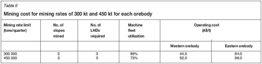
The cost analysis was conducted on operating a 10 t LHD unit together with the preparation and production work required to keep ore available to these units during an entire quarter. Details of this costing exercise are beyond the scope of this paper. For a mining rate of 300 kt per quarter, a mining cost of A$44 per ton was determined for the western orebody. Because the eastern orebody is located at depth in a highly stressed environment, the additional ground support and other features required to maintain an open sequencing regime is calculated to increase mining costs to A$84 per ton. The increase in the mining rate to 450 kt adds A$8 per ton and A$12 per ton to the previously established mining costs for the western and eastern orebodies respectively, which increases the costs to A$52 per ton and A$96 per ton. Table II provides a summary of mining costs and LHD requirements that formed the basis for this investigation. These operating costs (OPEX) include all mining activities (for example, development, drilling/blasting, backfilling) within each orebody and the activities needed to haul the ore to the surface for processing.

Assumptions

The following assumptions were made to model production from this operation.

► During simulation, an availability of 87% was used for all LHDs. This figure was based on a mean time between failure (MTBF) of 55.6 hours and mean time to repair (MTTR) of 8.56 hours

► A discount rate of 10% was applied to appropriately reflect the risk associated with the project

► For the purpose of this analysis, a range of copper prices starting at A$5250 and increasing by A$500 increments up to A$9750 was used. The starting price of A$5250 was selected because most feasibility studies on copper projects conducted in recent years generally used prices between A$5000 and A$5500 per ton over the long term, although the price at the time of this study was approximately A$6500 per ton. The copper price boom of 2011 witnessed copper prices reaching almost A$10 000 per ton, and thus the final price investigated for mine planning purposes was A$9750 per ton Cu to reflect the price during the boom

► All internal development activities required to access all areas of the orebody were completed, and no prior production of any kind occurred from any stope. However, the development cost was included in the analysis

► The focus of this investigation is on the operating NPV that was achieved using an associated operating cost (OPEX). As such, capital costs (CAPEX) have not been included at this point; however, a simple comparison between any increase in the operating NPV and present value capital cost requirements associated with achieving the operating NPV will determine whether the corresponding capital expenditure can be justified.

 

Model formulation

The formulation comprised simulation and mixed integer programming models. The simulation model involved moving the mined material by LHDs and dumping it into orepasses, then conveying material on the lower level to the shaft point. A General Purpose Simulation System/Henrikson (GPSS/H) was used to determine the number of LHDs. The simulation results were then used to calculate operating cash flows associated with each stope using MIP. The MIP model was developed using A Mathematical Programming Language (AMPL) and then solved using CPLEX. This generated an optimized production schedule to produce an operating NPV at each commodity price and mining rate scenario.

The simulation model

The model consists of eastern and western orebodies, located at different depths from the surface, with the aim of simulating the number of LHDs that can haul 450 kt per quarter. LHDs load and haul ore and dump to the orepasses located 250 m from the orebody. The orepass drops material to the lower level, from where it is conveyed to the shaft point. In this paper, the simulation model considered the movement of the material from the production areas to the orepasses. The times needed to load a bucket, travel to the orepass, dump, and return to the loading point were used as input variables. Only a single LHD can load at a loading point and other LHDs arriving wait until the loading point is free. Similarly, only a single LHD is allowed to dump and no interaction occurs during dumping for LHDs from both sides of the orebodies.

A GPSS/H consists of multiple processes operating at the same time and provides the capability for these processes to automatically interact with one another. Objects may be sent between processes that share common resources and influence the operation of all processes. The representation of the object is known as a transaction. Transactions compete for the use of system resources. As transactions flow, they automatically queue when the resources are not free for use. A transaction represents the real-world system and is executed by moving from one block to another. Blocks are the basic structural element of the GPSS/H simulation language. In GPSS/H, more than 50 different types of blocks are available for use in modelling complex problems (Schriber and Brunner, 2011). Complete programming codes were created and the simulation was run with four times replications. A replication is a simulation that uses the experiment's model logic and data but its own unique set of random numbers; thus it produces unique statistical results that are analysed in a set of such replications (Schriber and Brunner, 2011). The execution of a run takes the actions at the current simulated time and then advances the simulated clock. These two phases repeat continuously until the end of the program. The written program used macros to code repetitive events, such as loading, tramming, and dumping, to reduce the size of blocks in the model. The simulation was run for three months and consisted of two shifts of eight hours each in a day for five days in a week.

Mixed integer programming model formulation

The MIP model is presented that was created to generate the optimal quarterly life-of-mine production schedules for each commodity price and equipment utilization scenario and to comply with all constraints.

Subscript notation

The following subscript notation was used to define the model in general terms.

T Long-term schedule time period: t = 1, 2, 3.... T

S Long-term stope identifier: s = 1, 2, 3.... S

H Mining rate identifier: h = 1, 2, 3.... H.

Sets

Data-sets were defined to aid in the formulation of constraints.

ß_sSet of eligible long-term periods in which stope s can commence production (between e_sto l_s)

ß_tSet of eligible stopes that can be in production in long-term period t

a_t Set of eligible mining rates h available in long-term period t

Y_sSet of eligible mining rates h available to each stope s adj_sSet of all stopes adjacent to and that share a boundary with stope s

tpb_tSet of periods that include all periods up to the current period t.

Parameters

Parameters representing the numeric inputs and conditions.

n_tPresent value discount factor for period t

V_t For all values

cf_sUndiscounted cash flow (A$) from each stope s

e_sEarliest start time for stope s

l_sLatest start time for stope s (may be the result of a geotechnical or infrastructure parameter that demands that stope s be completed by a certain period)

r_sExtraction reserve (t) for each stope s

sc_tShaft/LHD/truck fleet movement capacity (t) for each orebody in each period t

p_shLink between the potential mining rate h of each stope s and the period/s each mining rate is expected to be available once production on the stope is initiated; 1 = available, 0 = not available.

Decision variables

One binary variable reflected whether or not a stope enters products in a certain period.

w_st1 If production from stope s is scheduled for period t, 0 otherwise

g_ht1 If mining rate h is scheduled for time period t, 0 otherwise.

Objective function

The optimal schedule was determined by maximizing the NPV of all activities/stopes under consideration.

 

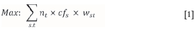
Note that taxation and depreciation were not included in this formulation but should be incorporated if necessary

Constraints

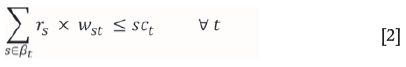
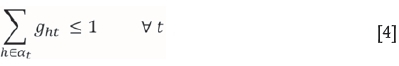
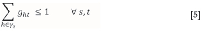
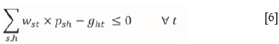
The practical limitations imposed by the sublevel stoping method over the long-term scheduling horizon were reflected through a series of constraints. Constraints [2] to [6] are considered resource constraints because they reflect the natural restriction of resource allocation throughout the mine during each scheduling period. Constraint [2] prevents the production of stope ore extraction from exceeding the shaft/LHD/truck fleet capacity for the overall mining operation or a specific part of it, including a particular part such as an orebody, in any long-term period. Constraint [3] enforces non-negativity and integer values of the appropriate variables. That a single mining rate was selected in each period was vital, as ensured by constraint [4]. Constraint [5] restricts each stope to a single mining rate in each period that it is in production. The rate of extraction of all stopes in any given period must match the extraction rate selected for that particular period, as enforced by Constraint [6].

Shaft / machine fleet ore capacity constraint

Non-negativity and integer value constraint

Single mining rate in each period

Single mining rate for each stope in each period

Mining rate match on all stopes in each period

Stope adjacency constraint

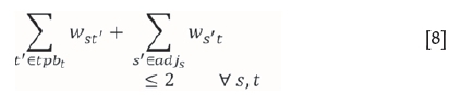
Fillmass adjacency constraint

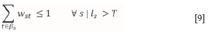
May mine constraint

Must mine constraint

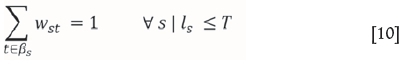
Constraints [7] and [8] are considered sequencing constraints because they reflect the safe and effective natural sequences inherent in the sublevel stoping method across the scheduling horizon. Constraint [7] ensures that simultaneous production between stopes that share a common boundary does not occur. Constraint [8] provides some geotechnical stability to stoping activities by limiting simultaneous adjacent production to two common boundaries before itself commencing production, and to a single adjacent side once having completed production to become a fillmass. Finally, constraints [9] and [10] are categorized as timing constraints because they reflect timing-related issues associated with each stope across the scheduling horizon. Constraint [9] ensures that stope production is initiated no more than once during the long-term scheduling horizon if the late start date occurs beyond the scheduling horizon. Constraint [10] requires stope production to commence at some point during the long-term scheduling horizon if the late start date falls within the long-term scheduling horizon. Note that this mathematical optimization model was used to carry out the evaluation when allowing for a variable mining rate. When a constant mining rate is maintained, constraints [4], [5], and [6] are not required.

 

Results and discussion

Simulation results

During model development, the model was coded to allow for the interactive input of variables at the start of the simulation run. As shown in Figure 1, a single 10 t LHD operating in either orebody is fully utilized and is expected to move 118 kt of ore each quarter. The addition of another LHD to the same orebody reduces total utilization to 96%, moving a combined 230 kt in each period. Adding a third LHD reduces the utilization of each machine to 89% with a total movement capacity of 320 kt and an excess capacity of 20 kt. Increasing each orebody mining rate from the current rate of 300 kt to the targeted rate of 450 kt indicates that overall targeted production from the entire operation could theoretically be sourced entirely from one of the two orebodies in each scheduling period. Given the different cost structure of each orebody as well as the copper grade profile, it was of interest to investigate if the higher mining rate would be utilized at any point across the commodity prices being analysed. Moving an LHD from one orebody to the other for part of the quarter causes a production delay; however, this was assumed to have a negligible effect on the simulation.

 

 

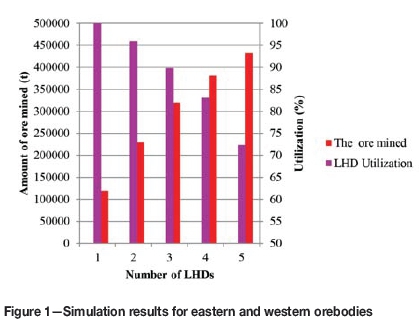
As shown in Figure 1, assigning four LHDs to the same orebody reduced total utilization to 83% and moved a combined 380 kt in each period. With five working LHDs, the total amount of ore moved was 432 kt and the average machine utilization fell to 73%. The 20 kt excess LHD fleet capacity from the initial orebody was assumed to be able to compensate for the 20 kt shortfall from the other orebody.

Therefore, three LHDs are required within one orebody to achieve the 300 kt mining rate, and two more LHDs are required to be in operation (a total of five LHDs) to achieve a mining rate of 450 kt.

Mixed integer programming scheduling

The MIP models for the purpose of optimal production scheduling (maximizing NPV) were written using A Mathematical Programming Language (AMPL). Based on the input costs and parameters previously mentioned, these models were solved using CPLEX 10.3. The solution process for each of the ten price scenarios evaluated was left to run overnight (approximately eight hours) and was cut short even if convergence to the optimal solution was not achieved. However, in all cases, a gap of less than 3.00% was achieved. In this case, production scheduling occurred in quarterly intervals and was limited to 60 quarters (15 years). Under each price scenario, full extraction from both orebodies was completed within the 60-quarter limit. Full extraction of each orebody was not expected at the lower copper prices of A$5250, A$5750, and A$6250 per ton Cu because the respective cut-off grades were higher than the grade of the lowest stopes. Full extraction from each orebody at each of the other copper price scenarios was not expected. Figure 2 compares the operating NPVs achieved when mining rates were limited to 300 kt and 450 kt in each orebody across each of the 10 copper price scenarios.

 

 

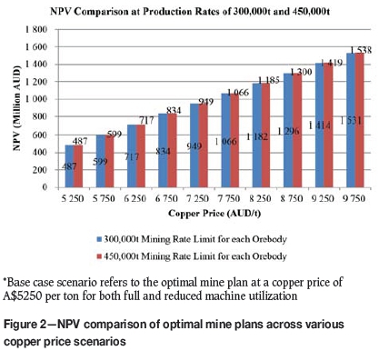
As shown in Figure 2, for the 300 kt mining rate, the A$5250 per ton copper price results in the lowest NPV of A$487.27 million. This NPV increases and ultimately reaches A$1530.64 million at the final copper price of A$9750 per ton. For the 450 kt mining rate, which had a higher mining cost, a similar trend was initially observed, with the lowest NPV of A$487.27 million at a copper price of A$5250. No differences were observed in the NPV between the 300 kt and 450 kt mining rates for copper price scenarios of A$5250, A$5750, A$6250, A$6750, A$7250, and A$7750 per ton. A slight increase of A$3.06 million, or 0.26%, in the NPV for the two mining rates emerged at the A$8250 per ton copper price. From this point, the difference in NPVs between the 450 kt and 300 kt mining rates increased as the copper price increased.

Table III compares the NPVs at each copper price for both mining rate scenarios. A copper price of A$5250 per ton under the 300 kt mining rate was used as a base case. The copper price increase from A$5250 to A$5750 per ton results in an increase in NPV of 1.49% for both mining rates. Table III also shows that no difference exists in the NPVs for both mining rates at the A$6250, A$6750, A$7250, and A$7750 per ton copper prices from the base case scenario. As the price increases to A$8250 per ton, a difference in the NPVs for the two mining rates begins to be observed. As is shown, the value attributed to the change in the mine plan at 450 kt increased to 4.97% from the base case scenario as opposed to 4.55% under the 300 kt mining rate. This result indicates that at this copper price, increasing the mining rate increases the NPV of the operation by 0.42% from the base case scenario compared with maintaining mining at a rate 300 kt. As the copper price increases further to A$9750 per ton, the NPV increases by 5.35% for the higher mining rate compared with 4.72% for the lower rate. Therefore, at the final copper price, the optimal mine plan utilizes the increased mining rate to create an additional 0.63% of value for the operation from the base case scenario compared with maintaining the same mining rate.

Changes to the optimal mine plan for the western (shallower) orebody compared with the eastern (deeper) orebody were analysed. It is apparent that each subsequent change to a higher commodity price favoured the higher grade eastern orebody, even though operational costs were also higher. This is reflected in the gradual decrease in the average period in which production took place from the eastern orebody stopes. Conversely, for the lower grade western orebody, the average period in which production from stopes took place increased as the commodity price was increased.

An analysis of these results shows that a short-term change in commodity prices added only the value provided by the increased margin associated with the new price. A longerterm price change should influence mining operations to continually update and adjust their mine plans to capture additional value under the new market conditions. These adjustments may include an increase in the mining rate. In this analysis, the capital costs of the working equipment were not included and therefore the evaluation was based on development and operating costs. For the lower mining rate at the final copper price, an NPV of A$1530.64 million was achieved, whereas at a higher mining rate, the NPV was A$1537.59 million. This represents a difference of A$6.95 million on a small and highly constrained example. It would be reasonable to suggest that a much higher difference would be achievable on a larger case. If the present value capital cost of purchasing the additional equipment in order to achieve the increased production rate at the higher commodity price is less than A$6.95 million, then moving ahead with this would be justified. This means that if the capital cost was more than A$6.95 million, an expansion in capacity cannot be justified. Each circumstance needs to be evaluated on a case-by-case basis in order to fully appreciate whether a change in market conditions warrants altering the mine plan to consider alternative mining rates. For a given mine configuration, a mine that considers increasing its mining rate beyond the rate that provides a high equipment utilization will most often incur increased mining costs. However, as this paper shows, even an increased mining cost can result in additional value if the additional quality of mill feed warrants this, particularly at elevated commodity prices.

 

Conclusions

In this paper we presented the NPV component that can be directly attributed to changes in mine plans as commodity prices vary under traditional mining rates with low cost, in comparison to more aggressive higher mining rates with higher costs. The results of the case study show the following points.

► For the 300 kt mining rate at the final copper price, the NPV was observed to increase to A$1530.645 million, whereas for the 450 kt mining rate, the NPV increased to A$1537.59 million

► As mining operations proceed to greater depths, increasing or maintaining mining rates may be beneficial, particularly in the case of increasing commodity prices, even if doing so results in a higher operating cost

► From an economic perspective, these results show that commodity price variations play an important role in the optimization of mine planning and design. A shortterm change in commodity prices adds only as much value as is provided by the increased margin associated with the new price. A longer-term price change should influence mining operations to continually update and adjust their mine plans to capture additional value under the new market conditions

► The combination of discrete event simulation and mixed integer programming can be used to provide a feasible solution to, and a better understanding of, the operational systems and to reduce the risk associated with selecting a system.

 

References

Banks, J., Carson, J.S., Nelson, B.L., and Nicol, D.M. 2010. Discrete Event System Simulation. Pearson Education, New Jersey.         [ Links ]

Brennan, M.J. and Schwartz, E.S. 1985. Evaluating natural resource investments. Journal of Business, vol. 58, no. 2. pp. 135-157.         [ Links ]

Barabady, J. and Kumar, U. 2008. Reliability analysis of mining equipment: A case study of a crushing plant at Jajarm Bauxite Mine in Iran. Reliability Engineering and System Safety, vol. 93, no. 4. pp. 647-653.         [ Links ]

Camus, J. 2011. Personal communication. 23 September.         [ Links ]

Caterpillar. 2009. Caterpillar Performance Handbook. Edition 39. Caterpillar Inc., Peoria, IL.         [ Links ]

DING, B. 2001. Examining the planning stages in underground metal mines. PhD thesis, Queen's University.         [ Links ]

Floudas, CA. 1995. Nonlinear and Mixed-Integer Optimisation: Fundamentals and Applications. Oxford University Press, New York.         [ Links ]

Govinda, R.M., Vardhan, H., and RAO, Y.V. 2009. Production optimisation using simulation models in mines: a critical review. International Journal of Operational Research, vol. 6, no. 3. pp. 350-359.         [ Links ]

Hall, B. and Stewart, C. 2004. Optimising the strategic mine plan - methodologies, findings, successes and failures. Proceedings of Orebody Modeling and Strategic Mine Planning, Perth, wA, 22-24 November 2004. Australasian Institute of Mining and Metallurgy, Melbourne. pp. 49-58.         [ Links ]

King, B. 2000. Optimal mine scheduling policies. PhD thesis, University of London.         [ Links ]

Lane, K.F. 1988. The Economic Definition of Ore: Cut-off Grades in Theory and Practice. Mining Journal Books, London .         [ Links ]

Mueller, M.J. 1994. Behavior of non-renewable natural resources firms under uncertainty: Optimizing or ad hoc. Energy Economics, vol. 16, no.1. pp. 9-21.         [ Links ]

McIsaac, G. 2008. Strategic design of an underground mine under conditions of metal price uncertainty. PhD thesis, Queen's University, Kingston, Ontario, Canada.         [ Links ]

Nehring, M., Topal, E., and Little, J. 2010. A new mathematical programming model for production schedule optimization in underground mining operations. Journal of the Southern African Institute of Mining and Metallurgy, vol. 110, no. 8, pp. 437-446.         [ Links ]

Salama, A., Nehring, M., and Greberg, J. 2014. Operating value optimisation using simulation and mixed integer programming. International Journal of Mining Reclamation and Environment, vol. 28, no. 1. pp. 25-46.         [ Links ]

Schriber, T.J. and Brunner, D.T. 2011. Inside simulation software: How it works and why it matters. Proceedings of the 2011 Winter Simulation Conference, Grand Arizona Resort, Phoenix, AZ, 11-14 December 2011. Jain, S., Creasey, R., Himmelspach, J., White, K.P., and Fu, M. (eds). IEEE, New York. pp. 80-94.         [ Links ]

Smith, L.D. 1997. A critical examination of the methods and factors affecting the selection of an optimum production rate. CIM Bulletin, vol. 90, no. 1007. pp. 48-54.         [ Links ]

Tatman, CR. 2001. Production-rate selection for steeply dipping tabular deposits. Mining Engineering, vol. 53, no. 10. pp. 62-64.         [ Links ]

Taylor, H.K. 1986. Rates of working of mines- a simple rule of thumb. Transactions of the Institute of Mining and Metallurgy (Section A: Mining industry), vol. 95. pp. A203-A204.         [ Links ]

Topal, E. 2008. Early start and late start algorithms to improve the solution time for long-term underground mine production scheduling. Journal of the Southern African Institute of Mining and Metallurgy, vol. 108, no. 2. pp. 99-107.         [ Links ]

Topuz, E., and Baral, S. 1988. A maintenance scheduling policy for mining equipment. Proceedings of the 17th International Symposium on Computer Applications in the Minerals Industry, Colorado School of Mines. Johnson, T.B and Barnes, R.J. (eds). SME, New York. pp. 155-160.         [ Links ]

Trout, L.P. 1995. Underground mine production scheduling using mixed integer programming. Proceedings of the 25th International Symposium on the Application of Computers and Operations Research in the Minerals Industry, Brosbale, Queensland, 9-14 July 1995. Australasian Institute of Mining and Metallurgy, Melbourne. pp. 395-400.         [ Links ]

Winston, W.L. and Goldberg, J.B. 2004. Operations Research: Applications and Algorithms. Thomson, Belmont, CA.         [ Links ]

Yap, A., Saconi, F., Nehring, M., Arteaga, F., Pinto, P., Asad, M.W.A., Ozhigin, S., Ozhigina, S., Mozer, D., Nagibin, A., Pul, E., Shvedov, D., Ozhigin, D., Gorokhov, D., and Karatayeva, V. 2013. Exploiting the metallurgical throughput-recovery relationship to optimise resource value as part of the production scheduling process. Minerals Engineering, vol. 53. pp. 74-83.         [ Links ]

Yearn, P. 1992. Economic optimization of mineral development and extraction. PhD thesis, McGill University.         [ Links ]

 

 

Paper received Sept. 2016
Revised paper received Jan. 2017