WITS SPECIAL EDITION - VOLUME II

 

Poor sampling, grade distribution, and financial outcomes

 

 

R.C.A. Minnitt

School of Mining Engineering, University of the Witwatersrand, South Africa

 

 

---

SYNOPSIS

This study examines the problems faced by open pit mine superintendents who make choices about how to direct their materials, either to the waste dump or to the mill. The paper explores the effects of introducing a 10% sampling error and a 0.9-times to 1.1-times sampling bias on positively skewed distributions for precious and base metals, negatively skewed distributions in the case of bulk commodities, and normal distributions as is the case for coal deposits. Parent distributions for each commodity were created on a 25 x 25 m grid using transformations of gold, iron ore, and coal data-sets, spatially based on a nonconditional Gaussian simulation. Ordinary kriging of grades for the three commodities into a 10 x 10 m grid provided the reference case against which the distributions with the sampling error and sampling bias for the commodities were compared. Imposing cut-off grades on the actual- versus-estimated scatterplots of the three commodities allowed the distributions to be classified into components of waste, dilution, ore, and lost ore. Ordinary kriging of values for each deposit type acted as the reference data-set against which the effects and influence of 10% sampling error and 0.9-times to 1.1-times sampling bias are measured in each deposit type. Indications are that the influence of error and bias is not as significant in gold deposits as it is in iron ore and coal deposits, where the introduction of small amounts of error and bias can severely affect the deposit value.

Keywords: sampling error, sampling bias, grade distribution, skewness.

---

 

 

Introduction

The effects of poor sampling and the financial implications for mining companies, traders in mineral assets, and sellers of metal as dore or commodities is documented in a number of studies, the most notable of which is that by Carasco (2004). He examined the financial impact of poor sampling practices in the Chilean copper industry and found that finacial losses due to poor sampling amounted to hundreds of millions of dollars over the life of a mining operation. Holmes (2004) examined the effects of correct sampling and measurement as the foundations of metallurgical balances, and found that revenues from the sales of large iron ore shipments may be profoundly affected by poor sampling practices. In South Africa the way in which sampling of in situ gold-bearing reefs affects the mine call factor has been an ongoing study since the disparity between the estimation of gold in the reef and the actual gold bullion produced was noted by early investigators such as Beringer (1938), Jackson (1946), Sichel (1947), Harrison (1952), and a number of others.

This study explores the ways in which misclassification of ore and waste due to the uncertainty in grade estimation has important economic consequences, particularly if a cutoff grade is superimposed on a metal grade distribution, as is normally the case. In addition, the study demonstrates how the gross value of a mineral deposit can be eroded as a result of poor sampling, taking into account the fact that mineral deposits of different metals, especially ferrous and non-ferrous metals, are characterized by the skewness of their distributions. Minerals characterized by the normal distribution for certain variables are also considered. The means by which the value of primary mineral deposits is affected as a result of the introduction of sampling error and sampling bias through poor sampling practise depends significantly on the nature of the metal distributions in the deposit.

The effects of poor sampling practise are examined for specific metals and commodities by introducing a 10% sampling error, and 0.9-times to 1.1-times sampling bias into otherwise unsampled mineral deposits. The error and bias are introduced on positively skewed, negatively skewed, and normal distributions for three main commodity types, namely gold, iron ore, and coal deposits.

 

Grade control and cut-off grade decisions

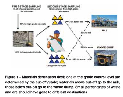
In most open-pit mining operations the pit superintendent is responsible for directing trucks leaving the pit to the waste dump or the mill, based on samples from blast-hole assays (Figure 1). Blast-holes are drilled on an ongoing 24/7 basis, keeping evaluation of the bench grade ahead of blasting and mining. Two problems arise for the pit superintendent, the first of which is due to the so-called 'support effect', sometimes also referred to as the volume-variance effect. The support effect refers to the size, volume, shape, orientation, and variability of samples collected for evaluation compared to that of the ore blocks or 'smallest mining units' (SMUs) that will actually be mined. Samples collected from typical blast-hole cuttings coming from a 31 cm diameter hole with a depth of 15 m, give a cone of rock cuttings around the drill steel with a volume of about 100 m³ which, at a density of 1.6 t/m³, weighs about 160 kg. After splitting, only 600 g of this mass will be sent to the assay laboratory, where analysts will probably use only a 30 g aliquot for the final assay. The mining block, by contrast, is a 7.8 x 8.8 x 15 m block with a density of 3 t/m³, containing about 2600 t of ore. The difference in support between the sample and the block being evaluated means that the variability in grade between the blast-hole samples is considerably higher than the variability between mining blocks, a characteristic referred to as the volume-variance effect. The volume-variance effect arises because of the difference in volume between blast-hole samples and the mining blocks, the variability in grade of the blast-hole samples and the mining blocks, and the way sample grades are applied to the estimation of SMU grades and tonnages. The larger the volume of the samples, the lower the variance. This problem is encountered in all mining operations where samples of relatively small mass are used to estimate the grade of much larger volumes of SMUs.

 

 

The difference in support size of the samples relative to the size of the blocks from which they are extracted leads to significant problems in terms of estimation, which in turn translate into considerable cost. Typically, bias observed due to the volume-variance effect changes the nature of the estimator from a perfectly straight line at 45° to a line with a slope that is considerably less than 45°, as shown in Figure 2.

 

 

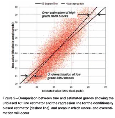
This means that if the sample grade (true grade) is below the average grade, the tendency is for the sample grade to underestimate the grade of the blocks. However, if the sample grade is above the mean then the tendency is for the face samples to overestimate the grade of the mining blocks (SMUs, Figure 2).

In most open-pit mines an operational cut-off grade is the principal criterion by which the superintendent makes his decision to send broken ore to the waste-dump or mill. Material with blast-hole grades below the cut-off grade is directed to a waste dump or low-grade stockpile, while broken rock with grades above the cut-off goes to the mill or a high-grade stockpile. The decisions to send material to the mill or the waste dump are based on incomplete information -the so-called 'information effect'. Lack of complete information is the root cause of imperfect decisions. The problem of the 'support effect' is worsened by the 'information effect' in that blocks of ground that should be sent to the waste dump are sent to the mill, and some blocks that should be sent to the mill end up being delivered to the waste dump, as shown diagrammatically in Figure 3.

 

 

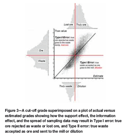
The histogram along the y-axis represents the true grade distribution for the deposit. The histogram along the upper x-axis refers to material that is truly ore; most of it is sent to the mill, but some of it is sent to the waste dumps as lost ore. The histogram along the lower x-axis refers to material that is truly waste; most of it is sent to the waste dump, but portion of it is sent to the mill as dilution.

The superintendent's problem is compounded by the fact that he is required to impose a cut-off grade on the materials mined, based on assumptions that are not true. The imposition of the cut-off grade presupposes that firstly, the decisions are based on the perfect estimator in the form of a 45° line in a plot of sample estimates versus block values, and secondly that the cut-off grade perfectly defines what broken rock should go to the waste dump and what to the mill.

In the day-to-day pressure of mining production, all the superintendent can do is base his decision on the estimated value he is given. According to Myers (1997) two errors are made; the first is an error of estimation because the value of waste material is estimated to be above the cut-off grade, and the second is an error of misclassification because the SMU is incorrectly classified as lying within the domain of revenue-generating ore. Such errors of estimation and misclassifi-cation arise because the decision about how to direct the ore is based on incomplete information. The first is a Type I error made when rock that is truly ore is rejected and sent to the waste dump, where it is lost to the value chain. The second is a Type II error made when rock that is truly waste material is accepted as ore, and is sent to the mill, where it dilutes the ore grade. The pit superintendent only has a 2D plan of the pit floor with blocks marked either above or below the cut-off grade. There are no blocks marked 'Ore, but actually waste', or 'Waste, but actually ore'. He must make a decision at the point where the cut-off grade is imposed; either ore or waste.

The category of 'lost ore' arises because truly economic ore is sent to the waste dump, where it is then 'lost' to the mining operation. The amount of lost ore is never known because it never adds value to the operation, it never appears on the balance sheet, there is no direct means of accounting for it, and it contributes to a low mine call factor. The only opportunity it may ever have of contributing to the mineral rents is at the end of the life of mine when the plant superintendent, desperate to fill the plant with material, resorts to using material off the low-grade stockpile. At one time South Africa's largest gold producer recovered 280 kg of gold per month from treating waste dumps (Brokken, personal communication, 2012).

The category referred to as 'dilution' arises because truly uneconomic rock is sent to the mill where it is processed as ore. Again, the amount of diluting rock is unknown, but it firstly appears indirectly on the balance sheet as a combination of higher milling and processing costs, and secondly it contributes to a lower mine call factor. Its overall contribution to the cash flow is negative. Quantifying the costs of dilution is difficult because the additional milling and processing costs are evenly spread across the entire stream of material arriving at the mill. This problem is amplified when milling capacity is constrained. The old adage 'a low-grade tonne should never keep a high-grade tonne out of the milt should be kept in mind.

The question that this research attempts to answer is whether these losses and additions to the mine revenue stream can be quantified in terms of sampling error and sampling bias, in terms of tons and grade, and in terms of dollars. This study aims to show that such quantification of the effects of sampling errors and sampling bias is indeed possible.

 

Methodology

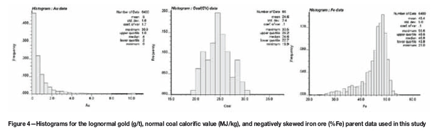
Grade distributions in a 1500 x 1500 m domain for three commodities gold (g/t), iron ore (%Fe), and coal (calorific value, MJ/kg) were created from parent distributions for each commodity, the histograms of which are shown in Figure 4.

The sampling distribution for each of the mineral deposit types examined here, gold, coal, and iron ore, are radically different and represent positvely skewed lognormal, normal, and negatively skewed distributions respectively. It is precisely the problem of sampling skewed distributions and the superimposition of error and bias on such distributions that this paper aims to investigate. The skewness of the distributions seriously affects sampling programmes and the overall estimation of the average grade of a mineral deposit. Even if we could eliminate all sampling errors and biases, the very nature of the distribution would mean that limited numbers of samples collected from positively skewed lognormal distributions, typical of precious and base metal deposits, will generally underestimate the average grade. For negatively skewed distributions, typical of bulk commodities such as iron ore, manganese, vanadium, and chromite, a limited number of samples will overestimate the mean, but in the case of mineral deposits with normally distributed variables, such as coal qualities and alumina, the mean grade of samples taken from these materials will generally be statistically correct.

The parent distributions were normal-score transformed and a transform table was generated for each commodity. This was followed by the creation of a single, simulated, nonconditional Gaussian distribution of 5 x 5 m pixels shown in Figure 5 using a spherical variogram model.

 

 

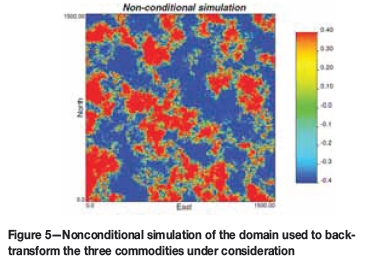
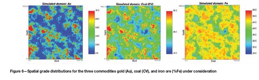
This single realization is the primary simulation from which three simulations of the commodities of interest, gold, iron ore, and coal, shown in Figure 6, were created. The domain file arising from the nonconditional simulation (Figure 5) was back-transformed using the normal score transform tables for each commodity (Au, Fe, and coal). This back-transformation produced three visually similar simulated distributions, which differ from one-another in grade distribution only (Figure 6). These three domains are made up of 5 x 5 m pixels in a 1500 x 1500 m domain and constitute the base case or reference distributions from which the 10 x 10 m block averages were created.

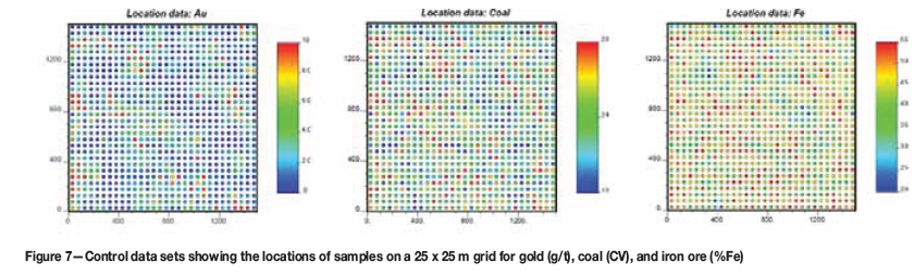
The 10 x 10 m block averages for each commodity of interest, created by block averaging the simulated distributions shown in Figure 6, were sampled on a 25 x 25 m grid. The locations of these samples for each of the commodities are shown in Figure 7. These constitute the control data-sets, containing no error and no bias.

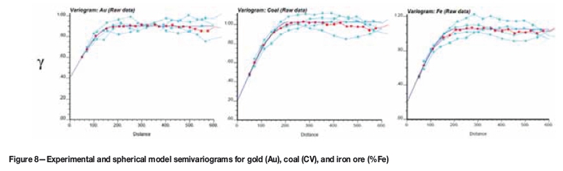
Experimental and modelled semivariograms for the data shown in Figure 7 are presented in Figure 8, and show a relatively higher nugget effect for gold compared to coal and iron ore.

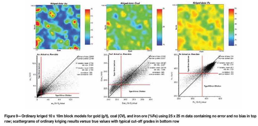
Ordinary kriging (OK) of the data shown in Figure 7 into 10 x 10 m blocks using the 25 x 25 m data and the semivar-iogram models (Figure 8) is shown in Figure 9. These three kriged models constitute the base-case reality containing no sampling error and no sampling bias, against which the effects of introducing error and bias can be compared.

Percentage sampling errors and multiplicative sampling bias are introduced into data-sets drawn from the 10 x 10 m block model for each commodity. This data is then kriged into 10 x 10 m blocks and the kriged outputs are compared against the reality base-case models shown in Figure 9.

 

Without sampling error and sampling bias

The daughter simulations for gold, coal, and iron ore at 5 x 5 metre pixels (Figure 6) were block-averaged into 10 x 10 m blocks and then sampled on a 25 x 25m grid (Figure 7) to produce an array of 900 points in each of the domains. Four sampling events, which drew the 900 samples on a regular 25 x 25 m grid from the 10 x 10 m block averages, were investigated. The first was a control data-set without the inclusion of any error or sampling bias and established the base-case reality against which the effects of sampling error and bias will be evaluated. The second, third, and fourth data-sets include 10% sampling error with no bias, a 10% sampling error with 0.9-times multiplicative bias, and 10% sampling error with 1.1-times multiplicative bias, respectively.

 

Figure 10

 

The actual 10 x 10m 'block average' control data-sets for gold, iron ore. and coal with no error and no bias are compared against the OK values in 10 x 10 m blocks in Figure 9. The effect of the differently skewed distributions is evident in the scattergrams. Lognormally distributed gold grades are concentrated in the lower left corner of the scattergram, negatively skewed iron ore grades occur mainly in the upper right of the scattergram, while normally distributed coal calorific values are evenly distributed across the scattergram. The effects of conditional bias are not evident in the gold or iron ore scattergrams, but are clearly evident for the coal scattergram, resulting in underestimation for low grades and overestimation for the higher grades (Figure 9, bottom row).

Typical exploration-stage or grade-control cut-off grades, 1.5 g/t for gold, 42 %Fe for iron ore, and 23 MJ/kg for coal (personal experience; Nel, 2013, personal communication; Steyn, 2013, personal communication) are superimposed on the scattergrams, and divide the scattergrams into quadrants containing ore, waste, dilution, and lost ore.

 

Introducing samping error and sampling bias

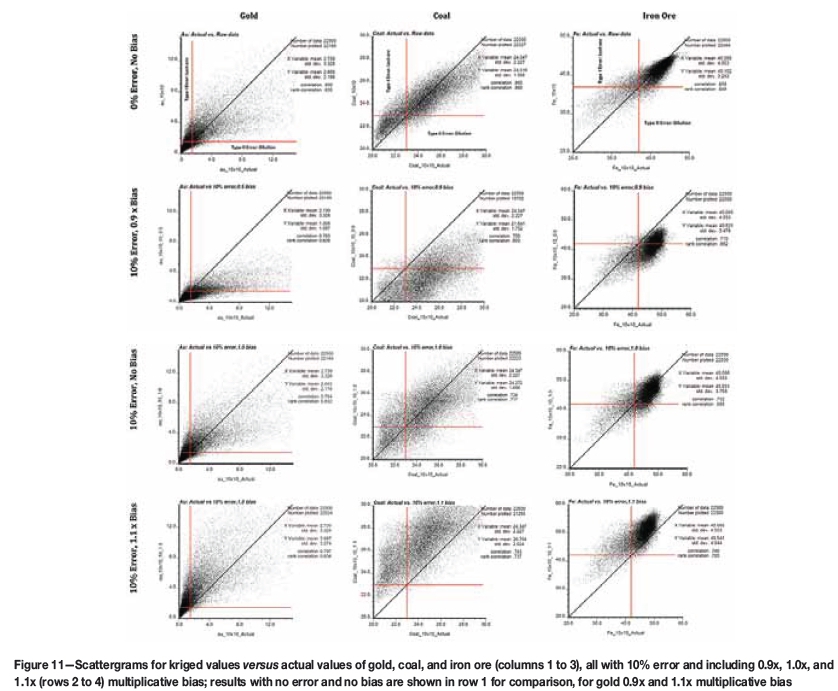
We now compare the kriged models in the scattergrams for the data-sets with and without the presence of sampling error and sampling bias. Introducing a 10% sampling error with no bias (third row, Figure 11) simply results in an increased spread of data in the scattergram. Error also increases the variability and decreases the correlation coefficient of the scattergram. The effect of 10% sampling error on changes in the tonnages and value of the deposits is negligable. The actual sample values versus OK results are presented in the scattergrams for gold, iron ore, and coal (columns 1 to 3, Figure 11). The first row of scattergrams in Figure 11 provide a visual standard with no error and no bias in the samples, against which the scattergrams with 10% error and differnt amounts of bias shown in rows 3, 4, and 5, can be compared.

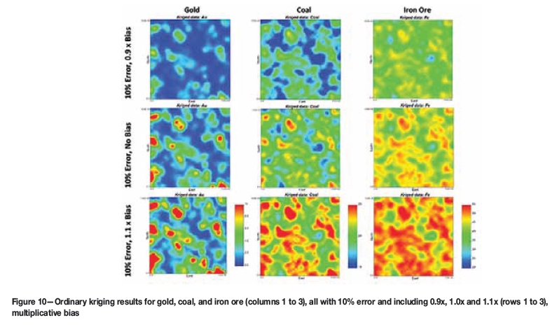
Although the kriged diagrams are colourful and show the columns with 10% error and different levels of bias, any visual interpretation is subjective. However, simple visual inspection indicates that the negative bias leads to undervaluation while the positive bias will result in overvaluation for the deposit. The effect of the error and bias is further emphasized in the scattergrams of actual grades against kriged results shown in Figure 11.

The effects of poor sampling are better seen in the scatterplots of the control data when compared against the data including error and bias. It is difficult to see the effects on the gold estimates, but the coal and iron ore estimates are clearly shifted in their positions on the scattergram. The effect of 10% error is simply to enlarge the distribution of the estimated points, while the negative bias shifts the points below the 45° line and the positive bias shifts the points above the 45° line. Again, these shifts are noteworthy, but of relatively little importance until we superimpose the cut-off values on the scattergrams.

Scattergrams in Figure 11 illustrate the difficulty that the pit superintendent faces, because the decisions he makes in sending broken rock to the mill or the waste dump can seriously affect the financial outcomes and profitability of the mining operation. The effects of bias on tonnage and deposit value are more obvious and severe than those of error. The sampling bias imposed on the already-introduced sampling error is multiplicative at 0.9 times and 1.1 times, 0.5 times and 1.5 times for gold. Bias shifts the cloud of points above or below the 45 degree line of unbiassed correlation. Inspection of Figure 11 indicates the points are shifted downwards for a 0.9x bias causing a significant increase in dilution, but a decrease in lost ore. In the same way a 1.1x bias causes a significant increase in lost ore, but a decrease in dilution, especially for iron ore and coal.

 

Evaluating the impact of error and bias on deposit value

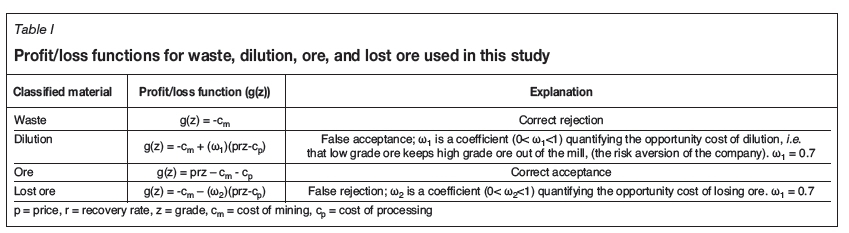
The value associated with mining waste, dilution, ore, and lost ore can be estimated through a profit/loss function. This provides a framework in which to evaluate the changing value of the four categories of mined materials affected by error and bias. Srivastava (1990) applied the loss function framework to evaluate the benefits of pumping solvent into an oil reservoir in order to improve recovery. He noted that any time an estimate involving over- or underestimation, rather than perfect information, is used to a make a decision, sub-optimality in the form of a loss will be incurred. He also noted that very often the error-induced loss is asymmetric and that the penalties for overestimation are different to those for underestimation. The application of profit and loss functions was carried further by Glacken (1997) and Verly (2005), who in a study of grade control classification of ore and waste undertook a critical review of estimation- and simulation-based procedures showing that misclassification due to uncertainty in grade estimation had economic consequences. The profit functions (g(z)) for blocks of waste, dilution, ore, and lost ore are listed in Table I.

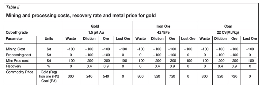
The profit/loss function is shown graphically in Figure 12 and provides a means of capturing the economic influence of mining the four classifications of material - waste, dilution, ore, and lost ore - in a single diagram. This allows the effects of error and bias to be seen in economic terms. The following mining and processing costs and cut-off grade parameters apply.

 

 

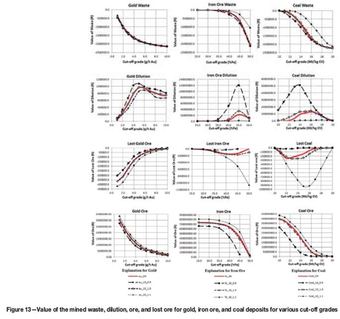
The profit/loss functions listed in Table I were applied for each class of mining material using the parameters listed in Table II in order to account for the characteristics of the material, its final destination, and the costs that the company incurs, or revenues it may lose as a result of a grade control decision. The curves showing the change in value for the four classes of materials - waste, dilution, ore, and lost ore - for gold, iron ore, and coal calculated in this way are shown in Figure 13. The standard reference for these plots is the OK result, which is shown in red in Figures 13 and 14.

A noteworthy feature of the 'Value of ore' shown in row four of Figure 13 is that the variability in value for gold is relatively small compared to that for iron ore and coal. In addition, the values for the commodities are concave-up for gold, concave-down for iron ore, and change from concave-down at low cut-offs to concave-up at higher cut-offs for coal.

 

Summary

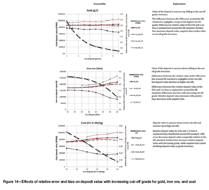
The relative effects of 10% error, 10% error plus 0.9x bias, and 10% error plus 1.1x bias on gold grades, iron ore grades, and coal CV values are summarized in Figure 14.

The effect of 10% sampling error on estimated deposit value is negligible for gold (about 0.3%), about 3.3% for iron ore, and 5.3% for coal. The effects of bias are asymmetric and significant with differences in estimated relative deposit value, as shown in Figure 14. The range in value due to bias in lognormal grade distributions for gold deposits is approximately 18%, for iron ore with negatively skewed distributions the range is about 47%, and for normally distributed CV values in a coal deposit the range in value is about 50%. Positive bias (1.1x) results in overestimation of value, whereas a negative bias (0.9x) results in significant underestimation of value with increasing cut-off grade. A positive bias (of the same magnitude as a negative bias) appears to have less effect on overvaluation than the negative bias has on undervaluation.

 

Conclusions

In order to protect the value in our projects from the influence of poor sampling, we need to ask three questions (Francois-Bongargon, 2013). Firstly we should ask 'How much?', as this relates to the mass of sample material required if we are to achieve required levels of precision, and the need to customize the sampling protocol through heterogeneity studies. Secondly we need to ask 'How?', as this relates to minimizing segregation and upholding correctness through application of appropriate technology to ensure appropriate precision and biases are eliminated. Thirdly, we should ask 'Why?', as this relates to the fact that this is the only way in which representative samples can be extracted and the economics of the deposit can be preserved.

This study highlights the fact that only by minimizing error, and in particular the bias, is there the possibility of minimizing the adverse effects of dilution and lost ore, both of which cost the mining company money that can never be accounted for. Lognormally distributed gold grades suggest that gold mineralization is less susceptible to the effects of bias and error than iron ore (negatively skewed grade distributions) and coal deposits (normally distributed grades for calorific value).

 

Acknowledgements

This study arose out of discussions with Professor Clayton Deutsch, Centre for Computational Geostatistics, University of Alberta, on research around the topic of cokriging and the representation of its appropriate benefits. The proposed research project was discussed with Professor Chris Prins, MinRED, Anglo American plc, who helped to refine the geostatistical work flow. Their contributions to this study are gratefully acknowledged. This paper is a modified version of 'Changes in deposit value associated with sampling error and sampling bias' presented by the author at the 6th World Conference on Sampling and Blending (WCSB6) held in Lima, Peru, in 2013 and published with the permission of Gecamin.

 

References

Clark, I. 2000. Practical Geostatistics. Ecosse North America, Columbus, Ohio.         [ Links ]

Glacken, I.M. 1997. Change of support and use of economic parameters for block selection. Proceedings of Geostatistics Wollongong '96. Baafi, E.Y. and Schofield, N.A. (eds.). Kluwer, Dordrecht, The Netherlands. Vol. 2, pp.811-821.         [ Links ]

Deutsch, C.V. and Journel, A. 1998. GSLIB, Geostatistical Software Library and Users Guide. 2nd edn. Oxford University Press. 368 pp.         [ Links ]

Francois-Bongarpjn, D. 2013. Segregation, the next frontier. Proceedings of the 6th World Conference on Sampling and Blending (WCSB6), Lima, Peru, 19-22 November 2013. Beniscelli, J., Costa, J.F., Dominguez, O., Duggan, S., Esbensen, K., Lyman, G., and Sanfurgo, B. (eds.). Gecamin, Santiago. p. 29.         [ Links ]

Minnitt, R.C.A. 2013 Changes in deposit value associated with sampling error and sampling bias. Proceedings of the 6th World Conference on Sampling and Blending (WCSB6), Lima, Peru, 19-22 November 2013. Beniscelli, J., Costa, J.F., Dominguez, O., Duggan, S., Esbensen, K., Lyman, G., and Sanfurgo, B. (eds.). Gecamin, Santiago. p. 89.         [ Links ]

Myers, J.C. 1997. Geostatistical Error Management, Quantifying uncertainty for environmental sampling and mapping. Wiley. 571 pp.         [ Links ]

Nel, F. 2013. Kumba Resources, Anglo American plc. Personal communication.         [ Links ]

Srivastava, R.M. 1987. Minimum variance or maximum profitability? CIM Bulletin, vol. 80, no. 901. pp. 63-68.         [ Links ]

STEYN, M. 2013. Exxaro Coal. Personal communication.         [ Links ]

Verly, G. 2005. Grade control classification of ore and waste: A critical review of estimation and simulation based procedures. Mathematical Geology, vol. 37, no. 5, July 2005. pp. 451-475.         [ Links ]

Wellmer, F.W. 1989. Economic Evaluations in Exploration. Springer-Verlag, Berlin.         [ Links ]

 

Paper received Mar. 2016
Revised paper received Jun. 2016