GENERAL PAPERS

 

Integrated optimization of stope boundary selection and scheduling for sublevel stoping operations

 

 

T. Copland; M. Nehring

School of Mechanical and Mining Engineering, The University of Queensland, Brisbane, Queensland, Australia

 

 

---

SYNOPSIS

The decreasing availability of resources amenable to surface operations has led to increasing numbers of underground mines, with trends indicating this will continue into the future. As a result, there is a need for additional optimization processes and techniques for underground mines, with many analogous methods having already been developed for surface mining. Current methods for design and optimization of stope boundary selection and scheduling mainly involve heuristic methods which focus on a single lever. Individual optimality may be approached, but globally optimal results can be obtained only by an integrated, rigorous approach. In this paper we review previous methodologies for stope boundary selection and medium- to long-term scheduling and highlight the need for an integrated approach. Previous integrated approaches are reviewed and an improved modelling system proposed for shorter solution times and greater applicability to mining situations. Randomly generated data-sets for gold-copper mineralization are used to investigate the model performance, describing solution time as a function of data complexity.

Keywords: integer programming, operations research, sublevel stoping, stope boundary selection and scheduling, underground mining.

---

 

 

Introduction

The increasing need for mineral resources is driving an increase in underground mines. Lower grade mineralization with larger amounts of overburden is becoming economically viable due to technological advances; however, the software and tools available for strategic underground mine planning are not well developed. Advances in the methods used to determine underground layouts and scheduling must occur to ensure underground mining is as optimized as open pit operations, as underground mining involves many more technical restrictions.

The process of determining stope boundaries and scheduling is an example of an aspect of underground mining amenable to optimization (Topal and Sens, 2010). The current industry standard for medium- and long-term planning for sublevel stoping (SLS) is to exclusively determine stope outlines and then determine an appropriate sequence and schedule accordingly. This process violates the concept of optimality as integrating the constraints imposed by pre-determining stope outlines does not allow for considerations in scheduling to influence boundary planning (Ataee-Pour, 2005). An integrated planning process that combines both stope outlines and scheduling would approach the optimal solution and hence generate more value for operations. This investigation specifically deals with the underground sublevel stoping (SLS). Other underground mining methods such as block caving, sublevel caving, and room and pillar mining have unique characteristics and therefore require specific stope boundary/production scheduling considerations.

This optimization problem has been the subject of research, particularly over the past five years, with current models requiring up to 31 hours for a solution to be found on computer systems that have the typical processing power of onsite technical services systems, on standard size data-sets (Little, 2012). Complexities arising from the technical constraints inherent to SLS include single fillmass exposure, extraction level alignment, and non-concurrent production. These constraints must be appropriately reflected in modelling this mining method. As such, the increasing number and nature of variables required to accurately model these constraints has a dramatic effect on solution time. Reducing the solution time by applying ideas from the field of operations research and mathematical programming would potentially allow current models to be implemented in industry and generate greater value for resource projects.

The current industry practice is to manually create stope boundaries and schedule extraction separately. The creation of a model that decreases computation time while still generating similar results to current models would drastically improve the planning process for SLS. Increases in NPV in comparison to manual methods have been quoted as high as 30% and with such a large margin for improvement, current practices would benefit from the outcomes of this project (Little, 2012). Increases in productivity for personnel involved in long-term scheduling would also be expected as a manual approach for a single scenario can take multiple planners longer than three weeks (Wang and Webber, 2012).

 

Operations research

Model formulation

Goldberg and Winston (2004) define seven steps for model formulation. The process highlights the fact that all mathematical models are idealized approximations of real-life problems and hence solutions that are found must be critically analysed, implemented, and evaluated. Taha (2006) also notes that the added complexity of a model in attempting to idealize as little as possible can be rewarding in respect of increasing the validity of results. The seven steps outlined by Goldberg and Winston (2004) are:

► Formulate the problem

► Observe the system

► Formulate a mathematical model of the problem

► Verify the model and use the model for prediction

► Select a suitable alternative

► Present the results and conclusions of the study

► Implement and evaluate recommendations.

Linear programming

Linear programming (LP) is an analysis technique that aims to maximize or minimize a linear function with a number of variables. These models consist of an objective, decision variables, and constraints. Decision variables are representations of the choices to be made that affect the outcomes of the problem approximated, while objectives are linear functions of decision variables that are to be maximized or minimized in order to determine the optimal solution. Examples include maximizing profit by choosing how much of a product of a particular type to make. Constraints are inequalities that enforce some limit on the model so as to ensure the solution to the model is applicable to real-world situations. As the name implies, these must also be linear. Scarcities of resources or machining capacity limitations are examples of constraints in a production setting. LP models can be represented in the general form:

Linear programs can be solved in multiple ways. Simple programs containing two or three variables can be solved graphically or analytically by substitution of equations; however, more complex linear programs require more specialized tools. The simplex method exploits the geometry of a polytope which represents the feasible region of a problem with the number of dimensions corresponding to the number of decision variables (Noncedal and Wright, 2006).

The solution at which the algorithm is terminated is proven to be optimal as the polytope is convex, and hence a path along edges to the optimal solution will always have an increase in the objective function. The representation of a problem's feasible region will always result in a convex polytope if the problem is bounded and the matrix representing the constraint coefficients is linearly independent (Noncedal and Wright, 2006). The computation time for this algorithm varies, as the number of edges that must be traversed varies according to the dimension of the LP problem, the location of the optimal solution, and the starting point that is chosen.

Variations of Dantzig's simplex method exist. The revised simplex method utilizes the same mathematical grounding but involves maintaining a basis matrix representation of the constraints. This reduces computation time due to the sparse nature of the matrices involved (Noncedal and Wright, 2006). Interior-point algorithms can be used on larger problems and exploit the geometry of the feasible region differently (Taha, 2006).

The advantages of LP are stated by Tiwari and Shandilya (2006), who highlight the fact that the range in which these types of problems can be solved allows for fast computation. The authors go on to state that the limitations of the method result mainly from the difficulty in representing problems, as many applications of mathematical programming require integer values or are difficult to represent in continua. Hence there is applicability to problems based in economics and production where continuous variables are well suited to the representation of real-world systems.

Integer programming

Integer programming (IP) is similar to LP in that models are formulated with objectives functions, constraints, and decision variables. The difference exists in the nature of the decision variables. IP problems require decision variables to be integers and hence the ability to model discrete situations. Integer variables are popular in modelling production planning, scheduling, and networks (Karlof, 2006). IP problems follow the general form outlined below.

Variables can also be limited to binary outputs. These binary variables can be used to represent 'yes or no' decisions; an example from a popular application is the Sudoku problem. Matrices of binary variables represent the location of a particular number, creating expressions for the puzzle's constraints that are simple to capture mathematically (Taalman and Rosenhouse, 2011). These problems are a subset of IP and are termed binary integer programming (BIP).

Due to the discontinuous nature of the variables in both BIP and IP, the feasible region of the problem cannot be graphically represented as a polytope. The solving of IP problems therefore requires the application of different algorithms. If an IP problem's variables are redefined to be linear, the problem is termed a linear relaxation (LR). The feasible solutions of an IP problem are a subset of the LR and hence many algorithms use the LR as a starting point for iterations (Tiwari and Shandilya, 2006).

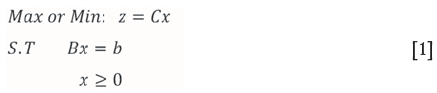
The branch and bound method is an algorithmic approach that uses a LR of an integer program to evaluate subproblems to determine the optimal solution of an IP problem. The process starts with solving the LR of the IP problem. If the solution consists of integers, then the process terminates and the optimal solution is found. If not, a non-integer variable is chosen and its bounding integers form constraints for the next sub-problem to be solved. This process continues until all possible solutions are investigated and the optimal solution is found. Figure 1 shows a branch and bound tree with the solutions of sub-problems from zero to ten forming the possible solutions to the initial IP problem.

 

 

Additional constraints can be added to an IP problem to decrease the region discrepancy of the LR. Another method for solving IP problems is the use of cutting planes. Cutting planes are derived from the optimal solution of a LR. Constraints in a Gaussian-reduced form are converted to integers and fractional parts, with the fractional then forming a new constraint. This constraint does not remove any feasible points from the IP problem, and changes the current optimal solution for the LR (Goldberg and Winston, 2004). Gomory (1958) shows that this process yields the optimal solution to the IP problem with a finite number of cuts.

The solution time for IP problems is highly dependent on the number of integer variables and the existence of any special structures instead of the number of constraints, as is the case with LP problems (Little, 2012). Increasing the number of constraints can actually decrease the solution time for IP problems by reducing the number of branches that can be investigated or reducing the feasible region (Hillier and Lieberman, 2001). IP is usually only limited in application due to the increased complexity of obtaining solutions, as this form of programming can model many real-life problems more accurately than LP.

Mixed integer programming

The combination of both continuous and integer decision variables in a programming problem is termed mixed integer programming (MIP). The applications of MIP extend to many areas. The solving of MIP consists of a combination of simplex-derived methods as well as IP problem-solving techniques such as branch and bound and cutting planes (Goldberg and Winston, 2004).

 

Sublevel stoping

Sublevel stoping is an underground mining method that involves the excavation of large blocks of ore in an unsupported fashion. This method is suited to steeply dipping, tabular orebodies of thickness between 50 to 100 m with strong, competent ore and host rock. Initially, stopes are developed with an extraction level and drill accesses, known as crosscuts (Figure 2). These development drives are offset vertically and are usually situated in the centre of a stope. Longhole drills are then used to create rings of holes within the stope envelope, which are then charged with explosive and blasted to fracture the rock. Ore is drawn down through the extraction level at the bottom of the stope. Once extraction has been completed, the void is then backfilled with material that may consist of waste, cement, and other aggregates. This process can be performed on multiple stopes simultaneously, within certain operational constraints (Darling, 2011).

 

 

Mine layout and design

The key aspects of underground mine layout that are pivotal to the project revolve around the limitation of when stopes are available for production. Haulage and access systems dictate when development can occur at different areas of the mine, and hence this should be reflected in modelling.

The use of a decline as the primary means of accessing the orebody favours production from stopes closer to the surface earlier, as these drifts can be developed before lower levels. If access is via conventional shaft-sinking, lower-level stopes may be favoured due to their closer proximity. Likewise, the choice of haulage system can also dictate these parameters in a similar way. Truck haulage systems may permit early production while other infrastructure is constructed, while shaft haulage will require initial construction of orepasses and underground crushers, hence preferences would vary according to the development method.

Stope shape also influences the value of underground operations. For thicker orebodies, where multiple stopes exist both along and across the strike, internal stopes may have regular outlines. At the point at which cut-off grade is to be defined, the profitability of a stope may influence its shape. A cut-off grade is defined as the point at which mineral concentrations become too low to be considered valuable and hence material below the cut-off grade is waste. Boundaries can be less regular to minimize dilution and as a result increase the profitability in comparison to a more regular outline. The level of geological confidence required in strategic planning to account for this is high and hence is not as applicable to this project, which seeks to maintain a more regular-shaped stoping envelope.

Production

SLS production processes involve multiple steps revolving around development, preparation, extraction, and backfilling. Initially, the extraction level and sublevel drill accesses are developed. The number of sublevel drives should be minimized as development is expensive in comparison to the cost of production drilling. Once these developments are completed, a slot raise or winze is driven at the initiating end of the stope; this serves as the initial void for production blasting (Sandvik, 2009).

Drawpoints are then constructed by drilling funnel shapes in the hangingwall of the extraction drive. Once the blasted material is removed, this will serve as another void for blasting and will channel broken ore from the stope (Nehring et al., 2012). After this, an initial slot is blasted to initiate breakage. The slot is smaller than future production blasts due to the space available for movement and the natural swell factor which occurs as material is broken. The stope is then blasted in stages and the blasted material extracted through the drawpoints. Ore can be transported by a combination of load haul dump units, orepasses, conveyors, rail systems, haulage trucks, and hoist skips (Darling, 2011).

A stope may remain empty for a period in which bulkheads are constructed within drives. These bulkheads ensure that the backfill material does not breach drifts. The fill mass is usually a combination of tailings and cement and is transported from the surface via a pipeline (Darling, 2011).

Stope sequencing and constraints

The geotechnical stability of openings underground dictates the way in which stopes can be extracted. There are a number of constraints that must be recognized when sequencing stope extraction so as to minimize the span of unsupported openings, decrease stress concentration on weak areas, and reduce the length of discontinuities in an attempt to maximize the stability and safety of operations. In order to accomplish these geotechnical goals, the following rules must be adhered to during production.

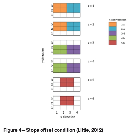
Stopes that overlie each other can create planes of weakness by having extended interfaces between fill mass and pillars. In order to avoid this hazard, stopes on adjacent levels must have offset outlines, so that these planes cannot form. Figure 4 demonstrates this.

 

 

 

 

In order to minimize the span of unsupported voids, stopes adjacent to a current production stope in any direction cannot be mined until the backfill material has cured. Concurrent production from stopes that are adjacent would increase the unsupported span and hence increase the risk of failure in the hangingwall, footwall, and backs. Production from stopes that share corners should also be avoided (Little, 2012).

The strength of fill mass is much lower than that of the surrounding country rock. As a result, if production from stopes exposes multiple sides of a backfilled stope, failure can be induced by the redistribution of stresses around the excavations. Therefore in order to avoid this potential for failure, production should allow only one side of a backfilled stope to be exposed at any one time.

Stope boundary optimization

While current industry practice is to perform this process manually, numerous methods are employed for stope boundary selection. Topal and Sens (2010) present a new method for determining optimal stope outlines. The method is rigorous and involves block model conversion, creating all possible stope outlines, evaluating envelopes of stopes for profitability, and choosing the most profitable stopes. The effect of different selection criteria in regard to profitability was investigated with total profit, profit per time unit, and profit per square metre used to determine the list of stopes to be mined.

The maximum value neighbourhood (MVN) algorithm is a heuristic approach to determining stope outlines from a block model. The method can be applied to three dimensions and is suitable for many different mining methods. It aims to find the maximum value for a stope that includes a block being interrogated. The algorithm starts with a definition of the largest stope size. Next, a set is populated that contains all the possible neighbourhoods, including the block in question. The economic value of each neighbourhood is determined by summing the profitability of each block in the neighbourhood, and the maximum is chosen. This process is repeated for other blocks with checks performed to ensure the same block is not included in multiple neighbourhoods (Ataee-Pour, 2005).

The moving cone method for open pit limit optimization is a widely used tool in the planning stages of surface operations. The floating stope algorithm is analogous to this method and aims to find the optimal limit of mineable ore in a stope envelope. A block is selected, with the inputs required being minimum stope outline and float increment. The outline is floated around the block, creating an inner envelope that consists of the highest grade stope and an outer envelope that encompasses all possible stope outlines. The stope outline to be chosen should be as close to the inner envelope as possible and fall within the outer envelope. The choice of stope outline is dictated by the optimization objective, such as maximum ore tons, maximum grade, or minimization of cut-off waste (Ataee-Pour, 2005).

The branch and bound technique utilizes type-two special ordered sets to determine the optimal starting and finishing locations for stope blocks in a row. Two piecewise linear functions are used to determine which blocks along a row should be included, and which should be excluded. The approach is implemented by commercially available software which includes data reduction, optimization, and graphical presentation (Little, 2012). The algorithm can be utilized only in one dimension, and hence the constraint of geometry and location of the row must be predetermined. While this tool is efficient, its limited application warrants the creation models of that can better approach optimality.

Scheduling approaches

The approach formulated by Manchuk (2007) demonstrates scheduling methods used in SLS operations once stope boundaries are determined. The process includes parameterization of stope attributes as well as of operations. Stope attributes include location, size, neighbouring stopes, and other economic factors, while operations are parameterized by task and the rate at which these tasks can be completed. Constraints in production are then applied. These include constant production, adjacency constraints, and resource allocation. The problem is then solved by a combination of simulated annealing and probabilistic decision-making.

As optimization over different horizons can provide only local optima, Nehring et al., 2012) investigated how an integrated schedule affects the NPV of an operation. Three models were derived - a medium-term schedule that optimizes production with the aim of maximizing NPV, a short-term production schedule allowing for machine allocations with the aim of minimizing deviation from a target grade to mill, and an integrated production schedule. The combination of both short- and medium-term optimization models showed significant results with an increase in NPV of 10% compared with manual scheduling methods, while the integrated model increased the NPV by 11% for a 100-stope conceptual study. The solution time for the non-integrated models is 110 seconds on a 2.40 GHz computer with 8 GB of random access memory.

 

Binary integer program formulation

Data structures

Creating a conceptual model that uses pre-processed stope data as opposed to generating stope data from blocks is a necessary step to reduce solution time. In doing so, purposefully structuring data to allow easy interpretation by the model minimizes processing time. The following steps outline the different aspects of creating the binary integer program inputs from block model parameters. Visual Basic for Applications (VBA) was used to perform this data processing.

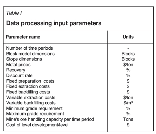
The following initial parameters are required to be filled before calculations can be done. These vary from financial to technical. Table I shows the required data.

 

 

Data processing

Each possible stope is investigated by evaluating the range of possible stope sizes and iterating through all the possible locations. The smallest increment that was investigated was the size of the blocks. Starting at the origin block of the model and with the smallest stope size, the boundary is stepped in a single direction until the extent of the block model is reached. Following this process in all directions, all possible stopes outlines are found. This is then repeated with as many stope sizes as input with beginning and end blocks written.

Once all possible stopes are determined, the block data is aggregated for each stope. Tonnage is calculated by summing individual block tonnages. Grade is calculated from a mass-weighted average of the blocks with value determined from the stope's containing metal. These are calculated using fixed and variable parameters. Stopes of negative value are removed in order to reduce model load. Removing the negatively valued stopes would not reduce the optimality of the solution as there is no way to increase NPV by including these stopes.

After removing negatively valued stopes, inter-stope data is formulated. Binary matrices are calculated according to a set of rules that determine which stopes are adjacent or cannot be in production with other stopes. A stope is chosen and compared to all other stopes. If the stopes being compared are on the same level, share an adjacent boundary, and do not have any common blocks, then the stopes are written as adjacent. For violation relationships, if the compared stopes have offset extraction layers, align for vertical planes of weakness, or share common blocks the stopes are written as violations. Supplying this data to the model allows for simple and systematic constraint application. From a computing point of view, the binary input of variables allows for faster computing than reading and referencing larger data labels.

After the data processing, stope data is amalgamated and saved. Each entry involves an identification index number, tonnage, grade, value, and extraction level. The value of each stope is output as a set of values corresponding to production in each time period. This allows for simple formulation of NPV and ensures the objective function remains linear. All data is written to a text file.

Binary integer program formulation

Mathematical formulation of the model involves multiple stages of compilation in order to optimize stope outline and scheduling simultaneously. The model aims to replicate real-world scenarios by selecting the most appropriate stope boundaries and locations in combination with time to produce and when level access should be developed. This is demonstrated in the way of binary decision variables.

The following sets and data are used in model formulation:

N_n   Set of all stopes indexed by n (or s)

T'_t  Set of all time periods indexed by t (or a)

L_l   Set of all levels indexed by l

G_g  Set of all metals contained by orebody indexed by g

Tm_t  Set of all time periods less one

Lm_l   Set of all levels less one

Ad_jns   Binary collection of data, 1 if stope s is adjacent to stope n, else 0

Viol_ns  Binary collection of data, 1 if stope s cannot be produced with stope n, else 0

Ton_n  Set of tonnage of stope n

ZZ_n   Level of stope n's extraction layer

LV_lt   Cost of level development in time period t

MG_ng  Grade of stope n for metal g

TonLim   Tonnage throughput limit per time period

MMax_g   Maximum mill feed grade for metal g

MMing    Minimum mill feed grade for metal g

The model consists of four types of decision variable, all with a binary nature. Two represent the production of stopes while two are used to demonstrate level access. The production variables are shown as:

The two variables used in level development are structured in a similar way:

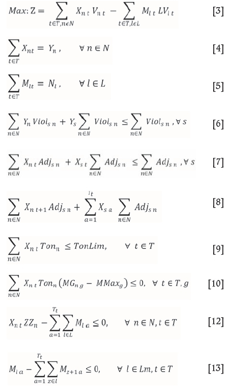
The objective function of the BIP is to maximize profit as shown in Equation [3]. This considers the profit from stopes and costs of level development. Equations [4] and [5] ensure that stopes are produced only once and that the summary variables are linked to the time-dimensioned variables. Equation [6] ensures no stopes that violate geotechnical constraints are produced or stopes with common blocks. Equations [7] and [8] constrain single fill mass exposure and non-concurrent production of adjacent stopes respectively. Equation [9] ensures production tonnage limits are not violated per time period, with Equations [10] and [11] ensuring blended metal grades are within specifications. Equation [12] ensures that production occurs only after level access is established, and Equation [13] ensures sequential development of levels from the surface.

 

Binary integer program performance

Model validation

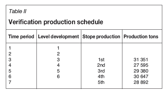
The model was verified by analysing the results of a 38-stope model with randomly generated financial parameters. A diagram demonstrating outlines is shown in Figure 5, with the production. This simulation had an NPV of $5.7 million. No violation of constraints was found, with visual verification of the production sequence showing that with the given development costs, stopes closer to the surface were more favourable for production.

 

 

The results of the model were compared to constraints previously outlined to ensure the selected stope boundaries and production schedule were valid. Systematically moving through the constraints:

► Stopes are produced only once if selected for production throughout the scheduling period

► No adjacent stopes are produced concurrently (this was further tested with a larger, tabular body and still held true)

► Single fill mass exposure is not exceeded

► No stopes have offset extraction levels

► No stopes cause vertical planes of weakness

► No stopes share common blocks

► Production tonnages are not exceeded

► Mill feed grade is kept within maximum and minimum requirements

► Level access is developed before stope extraction as required

► Level access occurs sequentially from the surface.

The implementation of the level constraint does not allow stope production to occur until after the level access is built. This is realistic in respect that it allows parallel production and development in the time periods after access and requires full development of a level before access. Table II shows the production and development schedule determined by the model to be optimal for the validation data-set. It shows that the level access constraint is not violated and production of stopes occurs in the time period after access has been established. It also shows that the production tonnage limitation was not violated.

 

 

Model performance with varying stope numbers

The model was run with varying stope numbers to predict solution time according to the input number of stopes to be solved. Solutions were obtained by using Python 2.7 with Gurobi Optimizer running on a computer with 8 GB of random access memory (RAM) and a processor speed of 2.00 GHz, utilizing all four of the processor's cores.

Figure 6 shows the number of stopes per model and the run time in minutes. Two variations of each model were run, one with a summary variable for stopes and levels and one without in order to compare processing times. A third reference from previous literature is included as a benchmark. This model (Little, 2012) was run with 4 GB of RAM and a 2.4 GHz processor and had a similar model complexity with regard to constraints and data. 289 stopes containing gold were evaluated with pre-processed physical and economic data with identical constraints in regards to mining, grade, and geotechnical limitations. The value of stopes was considered over multiple periods, however, and did not include level constraints.

 

 

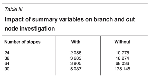
Both models, with and without summary variables, produced the same solutions for each data-set. This verification is required to ensure constraint spelling is correct. As models increase in complexity, it is expected that the results found for each model will begin to deviate. More intensive processing will be required for the model without summary variables and hence investigations may not reach a gap of 0%, whereas the other model will do so up to a certain number of stopes. Hence an improvement in model solution time is also an improvement in the size of models that can be investigated. The branch and cut algorithm used to find optimality demonstrates the number of solutions investigated in Table III.

 

 

Conclusions

The key findings include proof of optimality, reduction in solution time, and increases in applicability of model results. These are significant in mobilizing BIP as a method of planning and scheduling.

The model found the optimal solution for each case, solving each with a gap in solution space of less than 0.5%. Reaching optimality in a short time period is significant as it allows for higher NPVs to be obtained without reliance on manual methods. This allows multiple models to be run in different scenarios to investigate optimality, which cannot be done when manual methods are employed. It also removes the possibility for errors.

The methods of reducing solution time were successful in two ways. Firstly, by structuring data in ways that combine sets and allow for simple access by the model, processing time is reduced The use of binary sets to represent adjacency and violating relationships between stopes allowed for fewer constraints in the BIP and quicker data accessing as opposed to labels.

The second method of reducing solution time involves employing a summary variable to allow for constraints involving the whole production time-horizon to reduce the range of solutions to be investigated. It is more suitable for the violation constraint; for example, to consider the production schedule holistically rather than on a time period basis. Continuing with the violation constraint, a summary variable spelling would consider the subject stope variable in addition to a variable for all the stopes that cannot be produced. Without summary variables, the number of considerations increases by a factor of the time periods. Hence in the context for run solutions, the constraints could involve up to 25 times less variables.

The reduction in solution time as a result of using solution variables increased as data complexity increased. For the smallest models, nodes processed were reduced from 10 778 to 2058, reducing solution time from 13.09 seconds to 6.97 seconds. For the largest data-set assessed by both models, nodes were reduced from 175 145 to 5 087 for a solution time reduction of 5 664.38 seconds to 84.74 seconds. In comparison to previous work, a model run with similar computing hardware and stope numbers took 31 hours of processing time whereas with summary variables this was reduced to 135 minutes. The difference in these times increases the relevance of the project to industry as solution times approach acceptable limits for implementation in commercial software. A solution time of 31 hours would only be acceptable for academic investigations. While both processes reduce the risk of human error and allow for more iterations and scenarios to be tested, having up to 14 simulations in the space of one would allow for much greater productivity. Reducing the complexity of the model and nodes investigated would also mean that the limitations of computing hardware would affect only much larger models with the use of summary variables.

The addition of a level constraint allows for the results of the model to be more relevant to real-life applications. Although how this influences the relevance of model results cannot be quantitatively assessed, consideration for stope elevation adds valuable credibility and is a crucial factor in determining the optimal order in which stopes should be mined.

The implementation of this model or similar approaches would be an improvement on the current methods of manual formulation. The optimal solution is not guaranteed when relying on the experience of personnel and when stope outline and scheduling occur independently. Secondly, this work is an addition to the limited body of software for underground optimization. Its implementation would decrease the lag in development between surface and underground planning methods. Lastly, the model provides a basis for future work in the application of integer programming to other areas of underground optimization.

 

References

Ataee-Pour, M. 2005. A critical survey of the existing stope layout optimization techniques. Journal of Mining Science, vol. 41. pp. 447-466.         [ Links ]

Bullock, R.C. and Hustrulid, W.A. 2001. Underground Mining Methods: Engineering Fundamentals and International Case Studies. Society for Mining, Metallurgy and Exploration, Littleton, CO.         [ Links ]

Darling, P. 2011. SME Mining Engineering Handbook. 3rd edn. Society for Mining, Metallurgy and Exploration, Littleton, CO.         [ Links ]

Goldberg, J.B. and Winston, W.L. 2004. Operations Research: Applications and Algorithms. Thomson/Brooks/Cole, Belmont, CA.         [ Links ]

Gomory, R.E. 1958. Outline of an algorithm for integer solutions to linear programs. Bulletin of the American Mathematical Society, vol. 64. pp. 275-279.         [ Links ]

Hillier, F.S. and Lieberman, G.J. 2001. Introduction to Operations Research. 7th edn. McGraw-Hill, New York.         [ Links ]

Karlof, J.K. 2006. Integer Programming: Theory and Practice. Taylor & Francis, Boca Raton, FL.         [ Links ]

Little, J. 2012. Simultaneous optimisation of stope layouts and production schedules for long-term underground mine planning. PhD thesis, University of Queensland, Brisbane.         [ Links ]

Manchuk, J. 2007. Stope design and sequencing. MSc thesis, University of Alberta. 66 pp.         [ Links ]

Nehring, M., Topal, E., Kizil, M., and Knights, P. 2012. Integrated short and medium term underground mine production scheduling. Journal of the Southern African Institute of Mining and Metallurgy, vol. 112. pp. 365-378.         [ Links ]

Noncedal, J. and Wright, S. 2006. Numerical Optimization. Springer, New York.         [ Links ]

Sandvik. 2009. Sublevel stoping. Online, 8 July.         [ Links ]

Taalman, L. and Rosenhouse, J. 2011. Taking Sudoku Seriously: the Math Behind the World's Most Popular Pencil Puzzle. Oxford University Press, Oxford.         [ Links ]

Taha, H.A. 2006. Operations Research: an Introduction. 8th edn. Prentice-Hall, Upper Saddle River, NJ.         [ Links ]

Tiwari, N.X and Shandilya, S.K. 2006. Operations Research. Prentice-Hall, New Delhi.         [ Links ]

Topal, E. and Sens, J. 2010. A new algorithm for stope boundary optimization. Journal of Coal Science and Engineering, vol. 16. pp. 113-119.         [ Links ]

Wang, H. and Webber, T. 2012. Practical semiautomatic stope design and cutoff grade calculation method. Mining Engineering, vol. 64, no. 99. pp. 85-91.         [ Links ]

 

 

Paper received Oct. 2015
Revised paper received Mar. 2016