


Services on Demand
Article
 English (pdf)
 Article in xml format
 Article references
Indicators

Related links
-
 Cited by Google
 -
 Similars in Google
Share

 Permalink
Journal of the Southern African Institute of Mining and Metallurgy
On-line version ISSN 2411-9717
Print version ISSN 2225-6253
J. S. Afr. Inst. Min. Metall. vol.116 n.7 Johannesburg Jul. 2016
http://dx.doi.org/10.17159/2411-9717/2016/v116n7a8
PAPERS OF GENERAL INTEREST
Increasing the value and feasibility of open pit plans by integrating the mining system into the planning process
N. MoralesI; P. ReyesII
IDELPHOS Mine Planning Lab., Mining Engineering Department & Advanced Mining Technology Center, University of Chile
IITechnological Institute for Industrial Mathematics (ITMATI), University of Santiago de Compostela, Santiago de Compostela, Spain
SYNOPSIS
We present a model that allows us to consider mine production scheduling coupled with the mining system at different levels of detail: from the standard origin-destination approach to a network considering different processing paths. Each of these is characterized by variable costs, capacities, and geometallurgical constraints.
We then apply this model to a real mine, comparing the results with those obtained by traditional methodology: the destination of materials defined a priori, before computing the schedules, using standard criteria like cut-off grades.
As expected, using optimization to schedule and define dynamically the best processing alternatives shows a big opportunity for potential value improvement. However, the main result is that using only origin-destination and fixed cut-off grades may produce schedules that are not feasible when the actual constraints of the mining system are taken into account. Therefore, it is essential to include the considerations proposed in the planning process.
Keywords: mine planning, optimization, open pit, cheduling, multi-destination, mining system
Introduction
Mine planning is defined as the process of mining engineering that transforms the mineral resource into the best productive business. A central point of this process is the production plan, which is a bankable document that sets the production goals over the planning horizon (short, medium, or long) (Rubio, 2006). In turn, this production plan is supported by a production scheduling that indicates which part of the resource must be extracted in each period and what to do with these portions of the resource in order to reach the production goals indicated in the production plan.
In order to deliver a feasible production scheduling, the mine planning process must deal with complex issues like operational and metallurgical limitations, slope angles, stock handling, design, mining system selection, fleet considerations, etc. This means that it is not possible to construct the production scheduling in a single step considering all the elements involved, but that the process is split into different stages, which depending on the time horizon and level of decision, rely on different levels of information and must comply with different levels of precision and detail.
Among the relevant aspects that are traditionally left out by optimization tools for mine planning, it is possible to mention (Espinoza et al., 2013): optimal mine design of phases, roads, and operational space; equipment considerations like location, capabilities, and optimal fleet size; optimal processing capabilities; inventory management; and stochastic data. As the planning horizon decreases from long-term to shorter periods, the length of this list increases as it must comply with additional considerations of more detailed decision levels (see, for example, Newman et al., (2010) for a more detailed presentation of the different decisions levels).
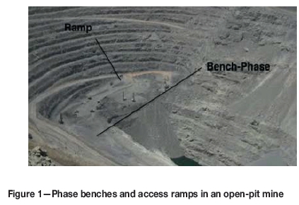
One example of the increasing complexity of the information and planning constraints that we address in the model used in this study is that long-term production scheduling is constructed without taking into account the variability of the ore content within a phase bench. Indeed, in long-term mine planning, large portions of material (called bench phases, see Figure 1 for a graphical example) are scheduled assuming a homogeneous distribution of materials within the bench. Indeed, the actual attributes of the rock (like grades or hardness) change within the bench and therefore, the availability of ore for processing is a function of the schedule within the bench, which in turn is limited, for example, by the location of the ramps and the type of equipment used in the mine.
A result of the example described above is that constructing medium- and short- term production scheduling can be very difficult, because the planner must comply with production goals set in longer-term decisions which are based on less restrictive constraints. Furthermore, there are very few computational optimizing tools to aid the short-term planner, so the process is a manual -trial-and- error procedure with an important time investment that consists of finding a feasible scheduling, leaving little room for optimality in terms of recoverable metal, fleet utilization, and reserves consumption among other items. Hence, at the end of the day, the short-term plans are unfeasible (within the parts of the mine scheduled for production) or the costs are higher than the optimal.
The approach that we propose aims to advance the solution of this and other issues related to short-term mine planning. For this, we integrate considerations related to the mine, but also elements related to the mining system downstream.
Mining system considerations
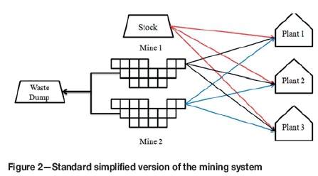
The standard way of looking at the mining system from a mine scheduling point of view can be illustrated as in Figure 2, in which material is evaluated in terms of the net profit with regard to a certain process choice. For example, the value of a block sent to the plant is different from the value of the same block sent to the waste dump. In fact, in longterm mine planning, this potential choice is reduced further on by using cut-off grades. Indeed, the actual destination of a block is chosen before scheduling simply by assuming that it will be sent to the most profitable process (plant or waste).
In this paper, we develop a different approach that aims for a more balanced (and hopefully more realistic) view of the mining system. We understand the mine planning scheduling from a pull perspective in which schedules are developed to maximize value and, therefore, must comply with considerations in terms of capacities, recoveries, and ultimately value.
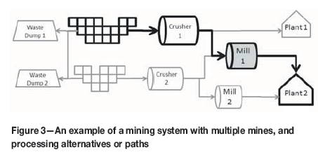
Our approach considers that there are many processing alternatives or processing paths. For example, as presented in Figure 3, an extracted block can go straight to a waste dump, or it can be sent to either of the two available crushers. In the latter case, the possibilities depend on the transportation system (whether the connection exists and its capacity) as well as the processing limitations of each facility (type of material, grades, etc).
The modelling we propose assigns material coming from the mine to the possible processing path. Depending on this decision, the corresponding material will have a certain economic value, but it will use certain processing resources like crushing time or transportation along the processing path.
For example, if one portion of material from a mine is assigned the highlighted path in Figure 3, then its actual economic value will be:
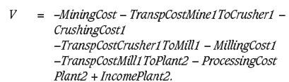
Certainly, the economic value in this case is different from that for any other path, and thus the optimal value will depend on the processing path choices.
Notice that the selection of the best processing path is not only dependent on the material itself, as assumed when using cut-offs to make such decisions. Indeed, the best processing path changes at each moment depending on the available processing capacities or the blending properties that impact the recovery at each plant. To account for these elements, we consider that:
►At each node in the mining system, a certain (possibly limited) number of resources are used. In this case, the resource is shared by all the paths going through the node. For example, in Figure 3 the total milling capacity at Mill1 is shared by the material coming from either Crusherl or Crusher2
►At each node in the mining system there may be blending constraints that limit, for example, the maximum content of certain pollutant. This constraint is applicable mostly at the plant nodes.
Mine considerations
Mine considerations are among the most studied in the literature on open pit scheduling. They refer to the technological aspects needed to comply with a certain slope angle required for the pit. Furthermore, they also refer to overall operation size, which translates into mining capacities.
In terms of the mine, we consider that the material is discretized into mining reserve units (MRUs) (we use the term reserve as the MRUs are already scheduled for extraction in the long-term plans). Each MRU may correspond to a block in the original block model or it can represent other structures, either larger (drilling polygons) or smaller (shovel buckets) ones. This depends on long-term schedules. Notice that the actual set of available MRUs for scheduling is an input for the model.
For each MRU, there are some attributes that must be considered in the mining system constraints. For example, nodes could have capacity constraints. In that case, those MRUs will have a tonnage attribute stating the maximum tonnage allowed.
MRUs are also related by precedences referred to the slope angle or accessibility constraints. Slope precedence constraints relate to the fact that in an open pit mine there is a minimum angle to ensure the stability of the pit walls, hence it is not possible to excavate vertically as much as desired. Accessibility precedences relate to the fact that in the short term, there are already ramps constructed, and extraction will start in those ramps and will be propagated through the bench. This is, indeed, overlooked in long-term planning because, as explained previously, scheduling is done at the bench-phase level of aggregation.
Related work
The strategic decision of determining the optimum final pit has been effectively treated using the Lerchs-Grossman algorithm (Lerchs and Grossman, 1965) or the Picard flow networks method (Picard, 1976; Cacceta and Giannini, 1986). These methods are based on a block model that characterizes a mineralized body only in terms of the economic value of each block and the slope precedence constraints. As a result, these models are very aggregated and ignore key elements like mining and processing capacities or the possibility of selecting the optimal block destination in a dynamic setting.
The problem of generating a production schedule in open pit mines has also been studied at different levels of detail. For example, Johnson (1968) introduces a mixed integer problem for scheduling under capacity, slope angle, and grade constraints. The mathematical formulation shares several elements with ours (processing and mining capacity, grade control, multiple periods and destinations, slope controls), but the focus is quite different. Johnson (1968) focuses on strategic planning and introducing the mathematical formulation. We are more interested in the impact of more complex models on the planning results.
The problem introduced by Johnson (1968) and variations of that method have been widely studied, because it has proven to be very difficult to solve in practical cases due to the size of the problem. For example, some papers that provide techniques to speed the resolution of the model are those by Cacceta and Giannini (1986, 1988), and more recently Gaupp (2008), Cullenbine, Wood, and Newman (2011), Bienstock and Zuckerberg (2010), Chicoisne et al. (2012); and others that propose heuristics are Cacceta, Kelsey, and Giannini (1998), Gershon (1983, 1987), or Dagdelen and Johnson (1986) and Whittle Programming (1998) for parametric methods. Nevertheless, all these studies have a different focus than ours, as they concentrate on the resolution of the problem.
Works that are closer to ours are Kumral (2012, 2015), which schedule blocks under slope constraints and capacity constraints (with upper and lower bounds) and where the model decides the final destination of the blocks. Kumral (2014) also considers bounds on the grades sent to the plant and uses conditional simulations to incorporate ore grade variability and compares the results using a priori cut-off grades (which is the standard procedure in mine planning) rather than allowing the model to decide such destinations. Kumral (2015) includes constraints to reduce production variation between consecutive periods. Both papers are, nevertheless, oriented to long-term scheduling, do not consider the short-term accessibility constraints included in this work, and focus on block destination and not alternative processing paths.
Regarding open pit block scheduling for the short term, Smith (1988) poses a mixed integer programming model that is responsible for block extraction scheduling in the short term, with the objective of maximizing the production of the material of interest, subject to certain constrains on blending, while ensuring a simple scheme of horizontal and vertical constrains without considering the presence of stocks. In the same line, Morales and Rubio (2010) present a model to maximize the production of metal in a copper mine, subject to certain geometallurgical constraints. Eizavy and Askari-Nasab (2012) present aggregation techniques to help solving a mixed integer model for short-term open pit mining. The model considered there includes, as ours does, stocks, blending, and capacity constraints, but with fixed block destinations and directional constraints in bench accessibility, which is very different from our approach.
Mathematical modelling
In this section we present the main notation and the mathematical formulation of the optimization model used in this work. A brief introduction to the mathematical model follows, and then a discussion about its use, limits, and potential extensions for real applications.
Notation
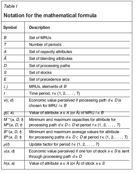
To begin, we consider a set of MRUs B = {1, 2, ..., N}. Time
is divided in T time periods, given in advance, hence the production is scheduled in periods t = 1, 2, . . . , T. Nevertheless, we do not assume that the periods have the same length.
There exists a set of processing paths D and we denote by d e D the potential processing paths in the mining system. In this way, the economic value perceived if MRU i is sent through processing path d Є D is denoted as v(i, d).
While the case study is short-term, we still consider that value of money over time is adjusted using an discount factor p(t) so that p(t) is the present value of a dollar perceived during time period t. For example, if the time periods had the same length (a year) and the yearly discount rate is a, then we would have that 
We consider two sets of attributes A and A. A refers to the block attributes that participate in capacity constraints like tonnage or processing times. A relates to the attributes that are averaged, like grades or pollutant contents. The value of attribute a Є A (or a Є A) in MRU i is denoted by g(i, a).
We model the precedence constraints as a set of arcs E  B x B, where (i,j) Є E means that MRU j has to be extracted before MRU i. (We provide extensive examples of this in the case study.)
We consider a set of pairs  where aℓЄ A and Dℓ
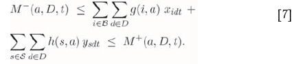
 D . For any (a, D) Є N, and for each t = 1, 2,..., T we are given a minimum capacity (thus a demand) M- (a, D, t) Є R
  and and maximum capacity M- (a, D, t) Є R
 . Similarly, we have a second set of pairs
 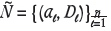 where aℓ and à and Dℓ
 D . For any (a, D) Є Ñ, and for each t = 1, 2, . . . , T we are given minimum and maximum average allowed values B-(a, D, t) Є R
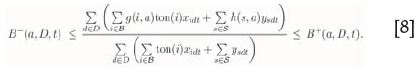
  and B+(a, D, t) Є R
 , respectively. For simplicity, we assume that attribute ton (i), the tonnage of MRU i, is the average of the weights. Extending the model to arbitrary weights is trivial.
The idea of having lower and upper bounds defined on sets of processing paths instead of bounds to each of the processing paths is that, as mentioned in the Introduction, the associated constraints aim to model limits at the nodes and, therefore, they will apply over the set of paths that go through them.
The model also considers a set S of stocks. Each stock can be seen as a MRU in the sense that all attributes a Є A have to be defined and we denote h (s, a) the value of the attribute a Є A for one ton of stock s Є S. We define h (s, a) analogously for ã Є Ã. Finally, we consider u(s, d) to be the value of sending one ton of stock s through processing path d Є D.
Note that the above definitions of value and attributes of stocks are per ton of material. This is because while stocks are treated similarly to MRUs, they are also different as they are not subject to precedence constrains. Moreover, it is possible to extract fractions of them and to send different fractions through different processing paths.
Given the above, in this model we use stocks only as possible sources of mineral, and not possible destinations. This will be discussed further.
A summary of this notation can be found in Table I
Mathematical formulation
This subsection introduces the decision variables, the objective function, and the constraints expressed in mathematical terms.
The decision variables are related to the decision whether to mine a given MRU, when to do so, and what processing path is chosen for that MRU; and similarly for material at the stockpiles. The constraints considered are those described above: capacity, blending, and precedence. Other constraints include scheduling constraints and constraints related to the nature of the variables.
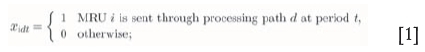
Variables
We consider, for each MRU i Є B, processing path d Є D, and period t = 1, 2, . . . , T, the variable
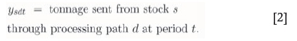
Similarly, for processing path d Є D, period t = 1, 2, . . . , T and stock s Є S:
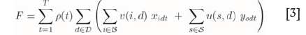
Objective function
The goal function considers the overall gain obtained from extracting and processing the MRUs, discounted over the planning horizon:
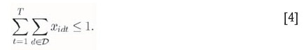
Constraints
Finite mass-The following constraint simply ensures that each MRU is processed at most once and sent through at most one processing path. For all MRU i Є B:
Similarly, for each stock s Є S.
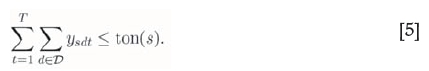
where ton(i) is the weight (in tonnage) of stock s Є S. Precedence constraints-As described before, these constraints are encoded in sets of arcs. They read, for each t = 1, 2, . . ., T and for Є E:

Capacity-For any time period t = 1, . . . , T and (a, D) Є N, we have that:
Blending-For any time period t = 1, . . . , T and (a, D) Є N, we have:
In the actual formulation of the problem, we transform these constraints to their equivalent linear representation.
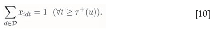
Scheduling constraints-We also consider several constraints that allow fixing or limiting the schedule of the MRUs. This is useful, for example, to construct heuristics for resolution of the problem or to compare the solutions obtained with other approaches (see later for examples). For this, we consider for each MRU i, time periods τ-(i), τ +(i) {1, 2, . . ., T}
where MRU i cannot be extracted before τ-(u) and has to be extracted by period τ+(u).
These constraints read:

and
Additional comments on the model
Capacity or blending constraints that affect specific material sources
The above formulation can be used, for example, to impose capacity or blending constraints that apply only to a certain set B  B of MRUs. For this, it suffices to create an attribute āsuch that g(i, ā) = 0 if MRU i /Є B. In this way, the MRUs outside B do not participate in the capacity or blending constraints. An example of this is the simulating the assignment of loading equipment to certain parts of the mine (see below for more details). The same technique can be used, for example, to impose capacities on the stocks.
Fixing or limiting MRU destinations or processing paths Similarly to the example above, by creating dummy attributes, it is possible to place a restriction such that MRUs in a given set B  B (and/or from given stocks) are not sent through a certain processing path d Є D.
Using the above two techniques it is possible preset the processing paths for certain MRUs or, for example, to fix cutoff grades for a given process path, or to force the condition that the material of a given stock follows some specific path.
Bench-by-bench extraction and minimum and maximum lead constraints
Precedence constraints can be used, for example, to model bench-by-bench extraction. This means that, within each phase, it is not possible to start the extraction of a lower bench unless the one immediately overlying it has been completely mined. For this, it suffices to mark as predecessors all the MRUs located in the bench phase immediately above a given one.
Another type of constraint that can be modelled using precedence constraints is related to the minimum/maximum distance (in benches) that must/can exists between two contiguous phases in the mine. For example, if we consider a minimum lead of three benches between hypothetical phases 1 and 2, this can be represented as imposing the requirement that MRUs in bench 1 of phase 2 are predecessors of MRUs in bench 4 of phase 1.
Optimizing equipment assignment
The model presented does not consider the capacities of the shovels or transportation fleet explicitly. Therefore, it cannot be used, in a direct manner, to optimize the assignment of loading equipment to different sectors of the mine over time. However, assignments of loading equipment can be modellec as capacities to specific parts of the mine or time periods (as described previously). Conversely, given a certain assignmen of the loading equipment, it is possible to model it by considering capacities in specific parts of the mine, at specific time periods. This approach allows us to use the model to optimize loading fleet assignments by looking at different potential scenarios.
Modelling ofstocks
In general, it is difficult to model stocks, because the attributes of the stocks (grades, tonnage) change with the schedule being computed. For example, one possible (but extreme) model consists of assuming that the grade of the stock is the average grade of its current content. This is highly nonlinear assumption, and thus difficult to solve. Even worse, it is not realistic, because mixing is not homogeneous, thus the stock ends up with layers of differen grade.
In the case of the model proposed in this paper it is possible to consider stocks as an input, as described before, but also as a possible destination for the MRUs. The actual scheduled process could then be split into several small stages: no mixing in the stocks occurs for a number of periods, then the stocks are updated accordingly to the material sent to them, and the scheduling process continues.
Other objective functions
An advantage of using a mathematical formulation of the problem is the fact that the objective function is very flexible. For example, it suffices to set p(t) = 1 in case of undiscounted cash flows. Moreover, the economic value coul refer only to costs that need to be minimized. Further on, considering the fact that different processing paths may lead to different metallurgical recoveries, it allows consideration o the case of maximizing the net mineral production.
Alternative formulations
Depending on the choice of variables, it is possible to write equivalent formulations of the problem above that may be better suited for computational purposes. For example, it is possible to use a by-formulation of the variables that allows the use of efficient solving schemes based on relaxation of certain constraints. A more detailed discussion on these topics can be found in in Espinoza et al. (2013).
Numerical experiences
In this section we introduce the case study used for applying the model described in the previous sections, as well as the experiments that were carried out.
Case study
For the case study, and in order to keep actual data confidential, we show only the information that is relevant for presenting the results. We have also normalized values like production tonnage, as described later.
The case study is of a porphyry copper mining complex consisting of two open pits or sub-mines, Mine1 and Mine2. The actual mining system consists of several crushers (including some in-pit), conveyor belts, intermediate stockpiles, and uses trucks for transportation. There are three different final processes, in some cases with more than one location each. Each block has more than 20 different processing paths.
All the alternatives mentioned previously are included in the modelling of the problem and its resolution, but for the sake of simplicity and to keep information confidential, we report for an aggregated system as shown in Figure 4. Note that standard planning procedures work at this level of aggregation, therefore it is also useful for comparison purposes.
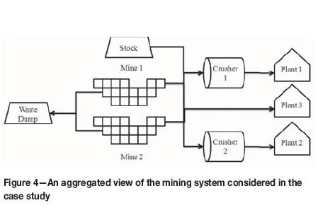
In our case study, the most profitable plant is Plantl, but it is also the one with more geometallurgical constraints. Plant2 and Plant3 have lower mineral recoveries and take longer to process the ore. Indeed, although no discount rate is applied between different periods in the planning, the economic values of MRUs sent to Plant2 and Plant3 are penalized according to the time required to produce the final product.
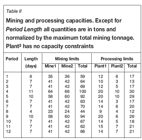
The planning horizon consists of a trimester, split into 12 periods with different lengths (from 4 days to 11 days). See, for example, Table II for details.
The capacity and blending constraints that affect the system are discussed below.
Capacity constraints
Capacity constraints are summarized in Table II. We are given three different mining capacities regarding the transportation limits: one upper bound for each mine (Minel and Mine2) and one for the entire mining complex. It should be noted that the joint capacity of both pits is larger than the global capacity of the mine, which allows some flexibility in the process.
Blending constraints
The case study included only one geometallurgical constraint, on Plantl, referring to a minimum Cu/Fe ratio of 0.5 for material fed to that plant in order to guarantee the efficiency of the process.
Precedence constraints
In terms of precedence constraints, we consider slope constraints, accessibility constraints at each bench, and bench-by-bench constraints.
Slope constraints
These constraints are given by a certain slope angle αand a tolerance height ∆z. Given two MRUs we consider that j is a predecessor of i if the mass centre of j lies in the upper cone with the vertex at the mass centre of i and angle a, and the vertical distance between these mass centres is at most ∆z. For example, in Figure 5a, MRU j is a predecessor of MRU i but jtis not, because although it is within the cone of angle a, it is farther than Δz above the mass centre of i.
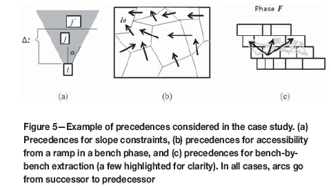
Notice that the threshold ∆zis used only to limit the number of arcs created in this way. Using this parameter is very common and does not mean that slope constraints are violated.
As seen in Figure 5, due to transitivity, the MRU jtis a predecessor of i even though the arc itself is not explicitly in E.
Accessibility within a phase bench
At each bench phase we consider at least one special MRU i0 representing the location of a ramp (see Figure 5b). Then, from this MRU i0, we compute the shortest Euclidean path that goes through MRUs in that bench phase, and add the precedence constraints accordingly. This allows us to guarantee that extraction within a bench phase (a) is propagated from the ramps, and (b) remains always continuous.
Bench-by-bench extraction
We also use precedence constraints to ensure that the extraction of a bench phase occurs only when the overlying bench has already been extracted. For this, we include precedence constraints between the MRUs of the lower bench and the MRUs at the top, as explained previously (see Figure 5c).
Notice that as these constraints relate only MRUs in the same phase, they cannot substitute slope precedences, which may affect MRUs from different phases.
Types ofschedule
The experiments generate production schedules using the optimization model and we compare them to the standard approach. The results of the experiments allow us to compare three scenarios: considering all the relevant short-term constraints (MODEL), with the MRU destinations defined beforehand (FIXED), or the standard approach (STD).
►STD corresponds to schedules and production plans obtained using the standard methodology available at the mine. In this case, the schedule is done at the beginning. The method takes into account the properties (attributes) of each individual MRU to define its final destination (and not the processing path that leads to it). Then the schedule is reviewed to satisfy mining and blending constraints at the final destination
►FIXED is a special case in which we preset the final destination of the MRU in the same way as in STD, and then schedule using the same considerations about mining and final destination capacities and blending constraints. In this case, the schedule used is the optimization model presented previously, but collapsing all the processing paths. Therefore, there is a unique aggregated path per destination, so as to mimic the STD case (See Figure 2 as an example)
►MODEL represents the resulting schedules and plans of our model. In this case, the economic values of the MRUs are computed for each possible processing path, and capacities and blending constraints are set at the node levels in the complete mining system. The scheduling process is carried out by the model, but also including the scheduling and processing path decisions as variables and not inputs.
As is mentioned in the description, schedules STD and FIXED do not take into account the mining system, but only the source and destination capacities. This is, indeed, the standard procedure in most mines (including this case study). This scheme is shown in Figure 2. In this case, intermediate nodes (including their associated capacities and constraints) are ignored in favour of an aggregated view that takes into account only the source and potential destinations.
For this reason, it was important to see whether these new elements introduced any changes in the resulting schedules or the assignment of MRU destinations. For this, we set two instances in which we considered the complete mining system but forced the model to comply with the STD and FIXED schedules, respectively. It was required to force the extraction of the MRUs at the same time periods of the corresponding schedules, and also to assign the actual processing path and comply with all the constraints along these paths.
Results and analysis
In this section we present and discuss the results obtained from the numerical experiments.
Firstly, we show the production plans obtained and some general conclusions. Next, we present the main result of this work, which shows the relevance of integrating the mining system in the mine scheduling. Finally, we analyse the differences in the production plans obtained.
Production plans
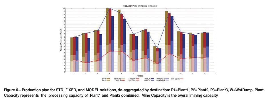
The resulting production plans are presented in Figure 6, in which we have de-aggregated the production for each schedule in terms of the final destination of the material.
We recall that the planning periods have different lengths, which translate into capacities that change from period to period.
Overall, these production plans show that the results obtained improve as more detail of the mining system is considered. More specifically:
►As expected, production schedules originating from optimization models tend to fulfill capacity constraints easily. However, the STD plan fails to comply with the mining tonnage constraint in some periods (see Figure 6, for example at periods 5 and 9). This is due to the fact that STD doesn't consider those constraints in the model
►FIXED and MODEL schedules tend to make better use of the processing capacities. For example, as there is no imposed capacity constraint on Plant3, both schedules make greater use of processing paths to that destination
►As there are no lower bounds imposed in the total mining tonnage, MODEL is able to produce higher production plans with less material extraction. For example, in periods 4 and 5 the total mined tonnage (stocks included) is about 85% of total capacity.
Economic value
The economic values of the three schedules are presented in Table III, normalized by the value obtained using the standard methodology. The numbers presented here must be regarded only as a reference because, as discussed later, there are several considerations to take into account.
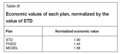
The scheduling FIXED (fixed destinations) results in a plan with value 44% higher than the traditional methodology (STD). Moreover, if we consider the destinations as part of the decision process (MODEL), the value is 14% higher than FIXED. In total, we obtain an increase of 58% with respect to STD.
The increase in value using optimization models for scheduling is expected and well documented in many case studies (see, for example, Caccetta and Giannini, 1988; Chicoisne et al., 2012). The increase due to selecting the optimal destination is also expected (see, for example, Kumral, 2013). Using an optimization model tends to produce superior results compared with manual or semi-automated procedures, within the corresponding model. Indeed, it is very important to note that these increases in value are not always reflected, because there are operational constraints not considered in the model. In our case it is important to take into account the following:
►STD is the only scheduling considered that satisfies the requirements of the planning procedure. Accordingly, it is the more realistic plan. Recall that STD considers only an aggregated level of constraints (for example, as in Figure 2) and therefore the model has less constraints than the corresponding MODEL version (as in Figure 4)
►Conversely, while FIXED and MODEL can be seen as good guides for constructing an operational plan, these models do not take into account all the complexities of a scheduling. Therefore, their economic values tend to be over-optimistic. Previous experiences comparing results from STD and FIXED show that about half of the increase by using a scheduling algorithm is lost in operational considerations (see Vargas, Morales, and Rubio, 2009a, 2009b for example). Then, we could expect a value increase of about 22%
► The economic value of MODEL has been evaluated under the same parameters as STD and FIXED, that is, at the origin/destination level using average costs. Nevertheless, the actual optimization process used costs to each processing path and the scheduling is optimized accordingly.
Despite the above considerations, we conclude that there is a huge potential value increase to be gained by means of optimized schedules. Furthermore, this approach allows the optimization model to choose the actual processing alternative for the material.
It may be also tempting to conclude that the potential of value optimization depends on scheduling instead of grade optimization. This requires further analysis because, as discussed in the following section, our experiments show that STD and FIXED cannot be applied because they do not satisfy the mining system constraints.
Scheduling considering the mining system versus not considering the mining system
We would like to point out how feasible it is to let the model choose the schedule. Thus, we set up an experiment taking into account the following considerations:
1. We used the same mining system modeling as in MODEL, i.e., we included all the intermediate nodes with the corresponding constraints
2. We included an additional constraint indicating that the extraction period of each MRU must be the same as in STD and FIXED
3. We allowed the model to schedule: the model chooses the processing path (and therefore, the final destination).
We expected that the model would produce a schedule with different choices for the destinations and with higher value. As it turned out, the resulting schedules were unfeasible. This means that there was no possible assignment of processing paths to the MRUs that would comply with the capacities and blending constraints (at the detailed mining system), but also respecting the schedule of STD or FIXED. Therefore, we conclude that these schedules were unfeasible from the very beginning.
We would like to stress that in the above experiment, the decision of which processing paths to use (and therefore destination) was made by the model. That is, even with this added flexibility the problem still remained unfeasible.
In the following sections we provide some analysis to illustrate how the schedules differ.
Changes in the schedule
The changes in the production plans presented in the previous section also suppose changes in the production schedule. Table IV shows how the FIXED and MODEL schedules make different decisions regarding the extraction time for individual MRUs. The rows of the table are separated for each mine and correspond to the following.
►Same-This corresponds to the MRUs that are scheduled at the same time period as in the STD case
►Schedule Before-This corresponds to the fraction of MRUs that were scheduled at a period strictly before the period in the STD case
►Schedule After-This is the fraction of MRUs scheduled for extraction at a period strictly after the period in STD
►New Schedule-This corresponds to MRUs that were not scheduled for extraction in STD, but are now scheduled at a certain period
►Not scheduled-This is the case of MRUs that were originally scheduled for extraction by STD, but now they are left unmined by the corresponding schedule.
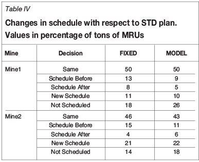
We observe from Table IV that, overall, the scheduled period remained the same in only about half of the cases, and that the decision for MRUs that were mined in all schedules is significant and accounts for about 20% of the tonnage.
What is more interesting is that there are very large differences in terms of the MRU being mined in the schedules. Indeed, if the destination decisions are the same as in the STD case (which is the FIXED plan), there is a difference of about 20% in terms of areas scheduled for mining, but this difference increases to 30% when destinations can be changed (MODEL case).
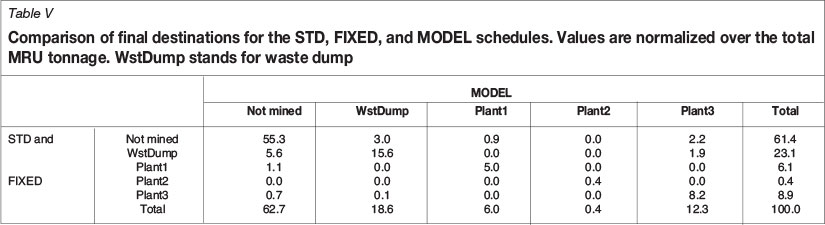
Changes in MRU destination
In order to compare the results obtained using a predefined destination for the MRUs with those obtained by letting the model choose the best option, we compare the actual destinations assigned to the MRUs in Table V.
Table V is constructed as follows. On each row we have the tonnage that the solution for STD or FIXED sent to the corresponding destination, but split according to the solution for MODEL. For example, the row Plant1 corresponds to material sent to Plant1 by FIXED. It indicates that 6.1% of the total mineral content was sent by the fixed destination to the plant (Total column), but the MODEL solution did the same for only 5% of this material, while 1.1% remained unextracted.
A first conclusion from Table V is that the there is a change of approximately 13% in the chosen destination of MRUs, as there are values that differ from zero outside the diagonal of the table. The only exception to this is the Plant2 destination. Indeed, both solutions send exactly the same 0.4% of the total tonnage to this destination.
We also observe that, while the total tonnage of material sent to Plant1 is not significantly different, MODEL mines less material by reducing the material sent to the waste dump while still increasing production, in particular the usage of Plant3.
Conclusions and future work
We have successfully modelled the mining system and extraction of an open pit operation under complex considerations and constraints of short-term planning that include accessibility, blending constraints, transportation and processing costs, slope angles, mining and processing capacities, etc.
We applied our model to a real case study, for which we conducted a series of experiments, in particular to compare the effect of using fixed rules to determine the destination of the blocks or MRUs (using, for example, cut-off grades) rather than leaving the optimal decision to the model.
The results show a high potential increase in the final value of a schedule under similar operational constraints, which is expected when comparing output from an optimization model with practice. Even better, the results also show an important potential in terms of using dynamic cut-off grades in order to optimize the final value of a mine operation, even under the hard limitations of volumes and design imposed by medium- and long-term decisions.
Even though the obtained schedule is not fully operational, it is close enough to provide a good guide for planners. Even more important, it allows the planner to make more robust decisions by exploring different scenarios. For example, although it is not reported in this article, we have used the model to study how the scheduling and processing path decisions change in the case of operational failure of the crushers, as well as considering different MRU definitions to study the impact of dilution of the scheduling process.
In terms of extensions of this work, we see at least the following research topics and applications:
(1) Improving the computation time, in order to be able to tackle more scenarios and larger case studies
(2) Improving the geometrical constraints imposed in the model so as to obtain schedules closer to operational ones
(3) Extending the models in order to deal with operational variability or geological and operational uncertainties.
Acknowledgments
This work was supported by CONICYT-Chile through the Basal Grant AMTC (FB0809). We would like to thank Edgardo Madariaga for his valuable technical support during this research.
References
Bienstock, D. and Zuckerberg, M. 2010. Solving LP relaxations of large-scale precedence constrained problems. IPCO Lecture Notes in Computer Science, vol. 6080. Eisenbrand, F. and Shepherd, F.B. (eds.). Springer. pp. 1-14. [ Links ]
Cacceta, L. and Giannini, L.M. 1986. Optimization techniques for the open pit limit problem. Journal of the Australasian Institute of Mining and Metallurgy, vol. 291. pp. 57-63. [ Links ]
Cacceta, L., Kelsey, P., and Giannini, L.M. 1998. Optimum pit mine production scheduling. Proceedings of the 3rd International APCOM Symposium on Application of Computers and Operations Research in the Minerals Industries, Kalgoorlie, Western Australia, 7-9 December. Vol. 5. Basu, A.J., Stockton, N., and Spottiswood, D. (eds). Australasian Institute of Mining and Metallurgy, Carlton, Victoria. pp. 65-72. [ Links ]
Caccetta, L. and Giannini, L.M. 1988. An application of discrete mathematics in the design of an open pit mine. Discrete Applied Mathematics, vol. 21, no. 1. pp. 1-19. [ Links ]
Chicoisne, R., Espinoza, D., Goycoolea, M., Moreno, E., and Rubio, E. 2012. A new algorithm for the open-pit mine production scheduling problem. Operations Research, vol. 60, no. 3. pp. 517-528. [ Links ]
Cullenbine, C., Wood, K., and Newman, A. 2011. Improving the tractability of the open pit mining block sequencing problem using a sliding time window heuristic with lagrangian relaxation. Optimization Letters, vol. 88, no. 3. pp. 365-377. [ Links ]
Dagdelen, K. and Johnson, T.B. 1986. Optimum open pit mine production scheduling by lagrangian parametrization. Proceedings of the 19th APCOM Symposium on Application of Computers and Operations Research in the Mineral Industry, Pennsylvania University, 14-16 April. Ramani, R.V. (ed.). Society of Mining Engineers, Littleton, CO. pp. 127-142. [ Links ]
Eizavy, H. and Askari-Nasab, H. 2012. A mixed integer linear programming model for short- term open pit production scheduling. Transactions of the Institution of Mining and Metallurgy. Section A, Mining Industry, vol. 12, no. 2. pp. 97-108. [ Links ]
Espinoza, D., Goycoolea, M., Moreno, E., and Newman, A. 2013. Minelib: a library of open pit mining problems. Annals of Operations Research, vol. 206, no. 1. pp. 93-114. [ Links ]
Gaupp, M. 2008. Methods for improving the tractability of the block sequencing problem for an open pit mine. PhD thesis, Division of Economics and Business, Colorado School of Mines. [ Links ]
Gershon, M.E. 1983. Optimal mine production scheduling: evaluation of large scale mathematical programming approaches. International Journal of Mining Engineering, vol. 1. pp. 315-329. [ Links ]
Gershon, M.E. 1987 Heuristic approaches for mine planning and production scheduling. International Journal of Mining and Geological Engineering, vol. 5. pp. 1-13. [ Links ]
Johnson, T.B. 1968. Optimum open pit mine production scheduling. PhD thesis, Universiry of California, Berkeley. [ Links ]
Kumral, M. 2012. Production planning of mines: optimisation of block sequencing and destination. International Journal of Mining, Reclamation and Environment, vol. 26, no. 2. pp. 93-103. [ Links ]
Kumral, M. 2013. Multi-period mine planning with multi-process routes. International Journal of Mining Science and Technology, vol. 23. pp. 317-321. [ Links ]
Lerchs, H. and Grossmann, I. 1965. Optimum design of open pit mines. CIM Bulletin, vol. 58. pp. 47-54. [ Links ]
Morales, C. and Rubio, E. 2010. Development of a mathematical programming model to support the planning of short-term mining. Proceedings of the 34th International Symposium on Application of Computers and Operations Research in the Mineral Industry (APCOM), Vancouver, Canada. CiM, Montreal. pp. 399-413. [ Links ]
Newman, A., Rubio, E., Caro, R., Weintraub, A., and Eurek, K. 2010. A review of operations research in mine planning. Interfaces, vol. 40, no. 3. pp. 222-245. [ Links ]
Picard, J.C. 1976. Maximum closure of a graph and applications to combinatorial problems. Management Sciences, vol. 22. pp. 1268-1272. [ Links ]
Rubio, E. 2006. Block cave mine infrastructure reliability applied to production planning. PhD thesis, University of British Columbia. [ Links ]
SMITH, M.L. 1988. optimizing short-term production schedules in surface mining - integrating mine modeling software with ampl/cplex. International Journal of Surface Mining, Reclamation and Environment, vol. 12. pp. 149-155. [ Links ]
Vargas, M., Morales, N., and Rubio, E. 2009a. Sequencing model for reserves extraction incorporating operacional and geometallurgical variables. Proceedings of Mine Planning, Santiago, Chile. [ Links ]
Vargas, M., Morales, N., and Rubio, E. 2009b. A short term mine planning model for open-pit mines with blending constraints. Proceedings of Mine Planning, santiago, Chile. Whittle Programming (Pty) Ltd. 1998. Four-X User Manual. Melbourne, Australia. [ Links ]
Paper received Oct. 2014.
© The Southern African Institute of Mining and Metallurgy, 2016. ISSN 2225-6253.

