


Services on Demand
Article
 English (pdf)
 Article in xml format
 Article references
Indicators

Related links
-
 Cited by Google
 -
 Similars in Google
Share

 Permalink
Journal of the Southern African Institute of Mining and Metallurgy
On-line version ISSN 2411-9717
Print version ISSN 2225-6253
J. S. Afr. Inst. Min. Metall. vol.116 n.7 Johannesburg Jul. 2016
http://dx.doi.org/10.17159/2411-9717/2016/v116n7a7
PAPERS OF GENERAL INTEREST
Optimizing open-pit block scheduling with exposed ore reserve
J. Saavedra-RosasI; E. JéivezII; J. AmayaIII; N. MoralesII
IDepartment of Mineral and Energy Economics, Curtin University, WA, Australia
IIDelphos Mine Planning Lab., AMTC & Department of Mining Engineering, Universidad de Chile, Santiago, Chile
IIICenter for Mathematical Modeling & Department of Mathematical Engineering, Universidad de Chile, Santiago, Chile
SYNOPSIS
A crucial problem in the open pit mining industry is to determine the optimal block scheduling, defining how the orebody will be sequenced for exploitation. An orebody is often comprised of several thousand or million blocks and the scheduling models for this structure are very complex, giving rise to very large combinatorial linear problems. Operational mine plans are usually produced on a yearly basis and further scheduling is attempted to provide monthly, weekly, and daily schedules. A portion of the ore reserve is said to be exposed if it is readily available for extraction at the start of the period. In this paper, an integer programming (IP) model is presented to generate pit designs under exposed ore reserve requirements, as an extension of the classical optimization models for mine planning. For this purpose, we introduce a set of new binary variables, representing which blocks can be declared as exposed ore reserve, in addition to the extraction and processing decisions. The model has been coded and tested in a set of standard instances, showing very encouraging results in the generation of operational block schedules.
Keywords: block scheduling, surface mining, open pit planning, optimization model, exposed ore reserve
Introduction
Open pit mines are characterized by high production levels and low operational costs compared to other exploitation methods. Unfortunately, when using this technique, material with poor economic value (waste) usually has to be removed to give access to more economically profitable material. Each block is characterized by its metal content, density, lithology, and other relevant attributes that are derived by using estimation techniques specifically designed to deal with the spatial nature of the mineralization. The value of a mine plan is thus determined by the value contained in the blocks that are extracted at certain periods and has a clear dependency on the block schedule, the order in which the material is extracted and processed.
Generally speaking, different problems are usually considered by mining planners for the economic valuation, design, and planning of open-pit mines, as pointed out by Hustrulid and Kuchta (2006); for example, the 'final pit problem', also called the 'ultimate pit limit problem', which aims to find the region of maximal undiscounted economic value for exploitation under certain geotechnical stability constraints. Another example is known as the open pit production scheduling problem, which aims to find an optimal sequence of extraction in a certain finite time horizon with bounded capacities (for example, extraction and processing) at each period and where the usual optimality criterion is the total discounted profit. A common practice for the formulation of these problems consists of describing an ore reserve via the construction of a three-dimensional block model from the orebody with each block corresponding to the basic volume of extraction, characterized by several geological and economic properties that are estimated from sample data. For this reason, the open pit production scheduling problem is also known as the block scheduling problem. Block models can be represented as directed graphs where nodes are associated with blocks, while arcs correspond to the precedence of these blocks, induced by physical and operational requirements derived from the geomechanics of slope stability. This discrete approach gives rise to huge combinatorial problems, the mathematical formulations of which are special large-scale instances of integer programming (IP) optimization problems; see for instance Caccetta (2007). Precedence between blocks is one of the most important sets of constraints, as the extraction process proceeds from surface down to the bottom of the mineralization. This idea applies to every block in the model: it is not possible to access a given block in a certain time unless the blocks that are above have already been extracted, because stability of the pit walls must be ensured. The amount of material to be transported and processed in each period is subject to upper and lower bounds, resulting from transportation and plant capacities, usually expressed in tons.
Regarding the block scheduling problem, a very general formulation was proposed by Johnson (1968, 1969), who presented a linear programming model under slope, capacity, and blending constraints (the latter given by ranges of the processed ore grade) within a multi-destination setting, i.e., the optimization model decides the best process to apply on a block-by-block basis. Unfortunately, the complexity of the model was too great to be solved in realistic case studies, and therefore the industry preferred an approach based on nested pits, computed as a parametrization of the ultimate pit solved with the algorithm proposed by Lerchs and Grossmann (1965) and subsequent improvements (see, for example, Picard, 1976; Hochbaum and Chen, 2000; Amankwah et al., 2014).
Caccetta and Hill (2003) proposed a model containing additional constraints on the mining extraction sequence and used a customized version of the branch-and-cut algorithm to solve it up to a few hundreds of thousands of blocks. Bley et al. (2010) used a similar model, but considering a fixed cutoff grade and incorporating additional cuts based on the capacity constraints that strengthen the formulation of the problem. This strategy was also used by Fricke (2006) in order to find inequalities that improve various integer formulations of the same model. Gaupp (2008) also reduced the number of variables by deriving minimum and maximum extraction periods for each block, therefore eliminating some of the variables and reducing the original MIP model size. Bienstock and Zuckerberg (2010) used Lagrangian relaxation on all constraints except the precedence constraints, reducing the model to the final pit problem. Chicoisne et al. (2012) focused on the case of one destination and one capacity constraint per period, developing a customized algorithm for the linear relaxation and a heuristic based on topological sorting to obtain integer feasible solutions. Cullembine et al. (2011) proposed a heuristic procedure using Lagrangian relaxation on lower and upper capacity constraints and a sliding time window strategy, in which late periods are also relaxed while variables of early periods are fixed incrementally. Lambert and Newman (2013) employed a tailored Lagrangian relaxation, which uses information obtained while generating the initial solution to select a dualization scheme for the resource constraints. Dagdelen et al. (1986, 1999) and Ramazan et al. (2005) worked on a model with fixed cut-off grades and upper and lower bounds for blending. Boland et al. (2009) proposed a different model, in which they aggregate blocks for the extraction decisions, including slope constraints, while the processing decisions are modelled at the level of individual blocks. Jélvez et al. (2016) used heuristics based on incremental and aggregation approaches in order to solve the open pit block scheduling problem. The model considers upper and lower capacity constraints, but the application considers only upper bounds. Zhang (2006) used a genetic algorithm combined with a block aggregation technique. Another approach is developed by Tabesh and Askari-Nasab (2011), who presented an algorithm that aggregates blocks into mining units and uses Tabu search to calibrate the number of final units; the resulting problem is then solved using standard IP algorithms. The aggregation technique is interesting, because it is based on a similarity index that considers attributes like rock type, ore grade, and the distance between the blocks.
The problem that this paper addresses is the design of a block schedule, but with the additional constraint of leaving enough exposed ore reserve that is readily available at the start of every period. Usually, once the phases are designed, their scheduling is adjusted so that there is always enough exposed ore to feed the processes for a few months. Unfortunately, these considerations are not included in the strategic optimization model that generates the phases and therefore operational delays may impact production. While this could be addressed using stocks, this is theoretically more complex (because of potential nonlinearity) and in practice requires material re-handling, which is more expensive and more difficult to track than material coming straight from the mine. On the other hand, as we show in this work, these constraints can be included in the block scheduling without these shortcomings. This may prove particularly relevant in the case of mines with disseminated or irregular ore distribution, and may be used as a tool to reduce stock sizes and therefore the operation footprint.
In terms of the model itself, as we will see later, the only cost to pay in the model is the introduction of new variables representing the exposed blocks and the corresponding new constraints, to be described in the next section.
Mathematical model
In this section the conceptual model is presented using an IP framework. It is important to stress that this new mathematical model is an extension of those considered as classical, but adds new variables and constraints that identify the blocks as exposed ore reserve.
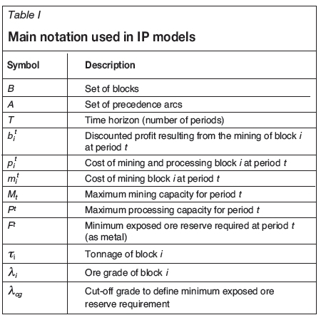
Let B be the set of blocks, and #B denote the number of blocks. Each block has a certain number of attributes such as tonnage and ore grade; these attributes permit the economic value of every block in B to be determined. The slope requirements for the set of blocks are described by a set of precedence arcs A  BxB, in such a manner that the pair (i,j) є A means that block i must be extracted by period t if block j needs to be extracted at period t.
In this model, a decision whether the extracted material should be sent to a processing plant or to the waste dump is included, thereby defining a variable cut-off grade. For each block i it is assumed that the tonnage τi, the ore grade λiand the net discounted value, given by  if block i is sent to processing plant at period t, and -
  if block i is sent to waste dump at period t, are known.
For every period t, maximum limits are imposed on the amount of material that is mined (Mt), and on the amount of ore that is milled (Pt). Moreover, in each period a minimum exposed ore reserve Ftmade available for the start of the next period must be guaranteed. For this, we will not allow every block to contribute to this minimum exposed reserve requirement, but only those above a certain cut-off grade λcg. In order to do this, it will be convenient to introduce the parameter
The reason for doing this is to give the model flexibility to choose mineralization from waste, but to prevent it from using many very low-grade blocks to comply with the constraint, therefore defeating the purpose of the model.
Table I summarizes the indexes, sets, and parameters used in the IP model.
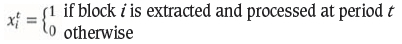
Three types of variables are used in the model, all of them binary. The first type is the variable associated to the extraction for processing purposes for each block:
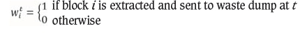
The second variable type describes the decision relating to the disposal of a block by sending it to the waste dump:
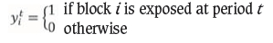
The third variable type is used to identify exposed blocks; throughout the paper it will be called the 'visibility' or 'exposure' variable:
The objective function for the model is the usual maximization of net present value (NPV). The formulation of the mathematical model is as follows:
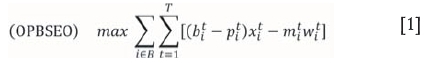
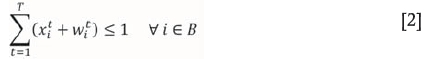
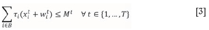

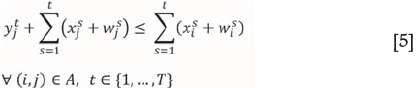

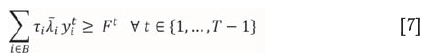
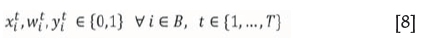
The objective function [1] represents the maximization of the cumulative discounted cash flow. Constraint [2] simply expresses that it is not possible to choose two different destinations for a block, i.e., a block can be sent either to process or to the waste dump, but not to both at the same period. Constraints [3] and [4] establish an upper bound on mining and ore production for each period. Analogous constraints related to other capacities of the system could also be established (e.g. water, energy, etc.). Constraint [5] is the usual slope constraint of open pit planning models, but written in a manner consistent with the identification of blocks that can be declared exposed for the start of the next period. Constraint [6] ensures that once exposed a block needs to be extracted and sent to the processing plant in the next period. Constraint [7] ensures that a minimum exposed reserve (in terms of units of extractable metal) must be available for the start of the next period (therefore, this is not imposed for period T). Finally, constraint [8] declares the nature of the variables involved in the model.
The model proposed here (which we name OPBSEO for 'open pit block scheduling with exposed ore reserve') contains #BxT new binary variables with respect to the standard open pit scheduling model (see, for example, CPIT in Espinoza et al. (2013)). The model has also #Bx(T-1) additional constraints of type [6] and T-1 constraints of type [7]. While in this work we focus on the model and the properties of its solutions, it is worth noting that the problem not only has more variables and constraints, but the structure is harder to exploit. In the CPIT problem (and also PCPSP), the vast majority of constraints correspond to precedences and they involve only two variables, one with coefficient 1 and other with coefficient -1. This corresponds to flow conservation constraints in a MAXFLOW problem, which allows the use of adapted methods like the BZ algorithm (see Bienstock and Zuckerberg, 2010). This is not the case for OPBSEO, as the precedence constraints do not have this simple structure.
It is also interesting to point out than an alternative way to approach the issue of exposed ore reserves is to use the standard formulation but with shorter time periods, so there is more control of the production at each moment in time. This means duplicating or triplicating the number of periods in which to handle ore reserve, and therefore implies that the total number of variables grows in the same order of magnitude, and in addition, this may produce a large number of requirements in terms of ore at every period, leading to infeasibilities.
Computational experiments
In this section a description of the application of OPBSEO to some instances is provided. The aim of these experiments is essentially to evaluate the performance of the proposed model and compare it with the equivalent IP model, but without exposed ore reserve requirements in terms of extraction geometries, exposed mineralization, and (to a lesser extent) NPV. In the first subsection the implementation of the model on a hypothetical two-dimensional orebody is described. Then two more realistic three-dimensional instances (block models and parameters) are presented, and finally the experiments on these instances as case studies are described and compared.
Example: two-dimensional data-set
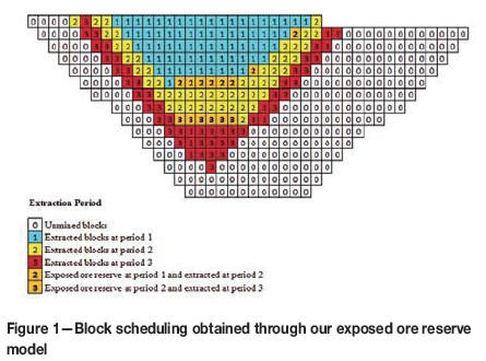
The instance considered here is a two-dimensional orebody (a slice of a three-dimensional deposit) that requires mining with a 45° slope angle. The block model contains 399 regular blocks, each of which has attributes such as tonnage and copper grade. Economic values associated with the extraction and destination (processing plant or waste dump) of the blocks are also given. The model decides the best destination for each block and defines exposed mineralization for each period while maximizing the NPV of the entire project. The planning horizon for this hypothetical case study is 3 years (considering annual periods) and the discount rate is set to 10%. Mining and processing capacities are fixed to a maximum of 4 Mt and 2.8 Mt per year, respectively. For each period, a minimum of 12 kt of exposed ore reserve is required and the minimum ore grade for a block to be considered exposed ore reserve is set to 0.3%.
The schedule obtained is shown in Figure 1. We can distinguish three important groups of blocks: unmined blocks, which are represented by code 0 (white); blocks mined in each period, encoded by numbers 1-2-3 (cyan, yellow, and brown, respectively); and exposed blocks within each period, in order to be mined and sent to processing at the next period (orange). An important aspect to highlight from the schedule is the geometry obtained at the bottom of the pit per period, which is quite satisfactory in terms of operational spaces.
Block models and parameters for two more realistic cases
The instances considered for this study were obtained from Minelib (Espinoza et al., 2013), a publicly available library of test problem instances for open pit mining problems, some of which correspond to real-world mining projects, making it very interesting for comparison. In our case, we used the Newman1 and Marvin instances described below, because they were more appropriate for our study in terms of the size of the instances (as mentioned before, the resulting problem is quite complex and required long computational times).
Newman1
The block model contains 1060 regular blocks. For each block there are attributes such as rock type, tonnage, ore grade, and economic values associated the destination of the blocks (waste dump or processing plant). In this instance the wall slope requirements are not given by an angle as usual, but to remove a given block, five blocks above must be extracted.
Annual periods with a yearly discount rate equivalent to an 8% are considered. The planning horizon is 6 years, but capacities permit completing the exploitation in 3 years. Mining and processing capacities are fixed to a maximum of 2 Mt and 1.1 Mt per year, respectively. For each period, a minimum of 5 kt of exposed ore reserve is required (as metal, calculated as tonnage multiplied by ore grade) to ensure production in the first half of the period, and the minimum grade for a block to be considered exposed ore reserve is set to 0.3%.
Marvin
This block model contains 53 271 blocks of 30 x 30 x 30 m, but this can be reduced when blocks that are not accessible are removed from the block model. The wall slope requirements are given by a 45° slope angle and by using seven levels of precedence above a given block. This deposit contains two metals of interest, copper and gold, and for each block there are attributes such as tonnage and grade. In order to consider a single-element deposit instead of multi-element one, we use a copper equivalent grade:
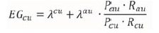
where EGcuis the copper equivalent grade, λcuand λauare the copper and gold grades, Pcuand Pauare the copper and gold prices, and Rcuand Rauare the copper and gold recoveries, respectively. The model contains some economic parameters that are used to obtain more realistic economic values for each block. The block value was obtained according the following expression:
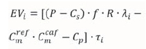
where EViis the economic value of block i and P is the price of the element of interest. Coefficients Cs,  , and
, and  are the selling, reference mining, and processing costs, respectively. The term
  is the block mining cost adjustment factor associated with the position (depth) of the block and ƒ is an appropriated unit conversion factor. R is the metallurgical recovery, λiis the equivalent ore grade, and
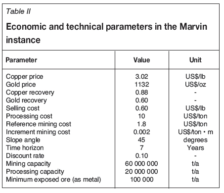
  is the tonnage of block i. We consider annual periods with a yearly discount rate of 10%, and the planning horizon is 7 years. Mining and processing capacities are fixed to a maximum of 60 Mt and 20 Mt per year, respectively. For each period, a minimum of 100 kt of exposed ore reserve (as metal) is required to ensure the first 4 months of production, and the minimum grade in order to a block for be considered exposed ore reserve is set to 0.25%. Table II summarizes the main economic and technical parameters.
Implementation/instance
In this subsection further detail is provided about the implementation of the exposed ore reserve model and other strategy to compare them. In the following cases no operational spatial constraints were considered. The following cases were implemented:
►Open pit block scheduling model with exposed ore reserve OPBSEO as detailed previously.
This is the main experiment in the article. The objective is to analyse the block schedule obtained in terms of extraction geometry, exposed ore reserve, and NPV. Newman1 and Marvin cases were implemented using the parameters explained in the previous subsection.
►Open pit block scheduling model without exposed mineralization, that is, OPBSEO but without binary variable
and without constraints [6] and [7]. This model is denoted as OPBS.
OPBS considers precedence constraints and limited mining and processing capacities only. Newman1 and Marvin instances were implemented using the parameters (if corresponding) detailed in the previous subsection. The comparison between OPBS and OPBSEO models is interesting because it allows the evaluation of the insertion within the same formulation of the exposed ore reserve concept.
In order to implement cases (a) and (b), PuLP was used (see Mitchell, 2009), which is a free open-source software written in Python that allows optimization problems to be set and solved with different optimization engines. In our case, we used GUROBI version 5.6.0 to solve the resulting IP models. Integer instances are solved up to a maximum 5% gap.
In all cases the resolution of the instances was performed on an Intel Core i5-3570 CPU machine with 16 GB running Windows XP version 2003. This machine has one processor with four cores, and is clocked at 3.4 GHz.
Results and discussion
Our interest is to evaluate the introduction of a new model with exposed ore reserve requirements, comparing the results obtained from OPBSEO and OPBS models, in terms of production plans, but also in terms of geometries and NPV. The results and discussion for two case studies, named Newman1 and Marvin, are presented.
Newman1 case study
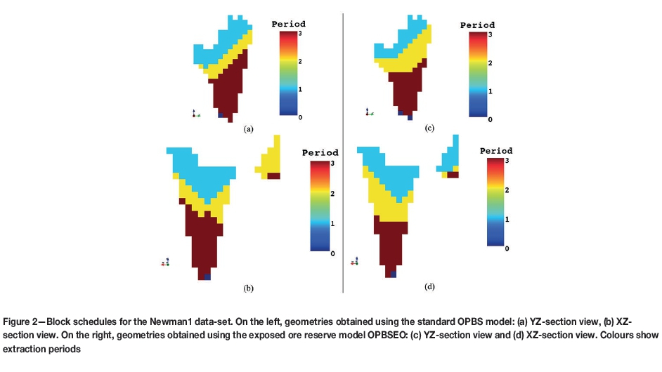
The pits obtained when scheduling the Newman1 case are shown in Figure 2, which presents XZ and YZ section views for both schedules, OPBS (left) and OPBSEO (right). The colours correspond to the periods at which the blocks are extracted. There are three extraction periods (cyan, yellow, and brown), unextracted blocks appear in dark blue.
First notice that this data-set has a very special shape. It is not a 'box full of blocks', but it consists of different disjoint parts. Also, the slopes at the borders are very steep. This is a property of the data-set as available in Minelib, and has nothing to do with the schedules. The most interesting property regarding the obtained geometries is that those with exposed ore reserve are better in terms of operational spaces and regularity. They are closer to a worst case and therefore suffer from fewer operational problems.
The production plans for the schedules are presented in Table III, which contains the following information: period indicates the year of the production, grade is the average grade of processed blocks, ore tons and total tons are respectively the processed and extracted material per period (in tons). Finally, exposed tons is the material exposed in that period and made available for the next period (in metal tons). The production plans are similar and both saturate the mining capacity, but the grades and exposed tonnages differ significantly. Indeed, OPBSEO extracts 9% less ore tonnage, but ensures that there is sufficient exposed ore for at least 6 months at the beginning of each period.
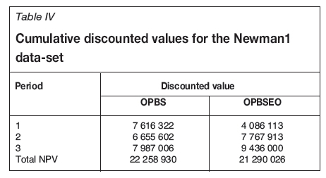
Regarding the NPVs (see Table IV), the block schedule computed using OPBS extracts blocks with higher grades as soon as possible, but OPBSEO has to deal with additional constraints of exposed ore reserves, which forces it to delay some high-grade blocks for future extraction. Still, the difference in NPVs is only 4% in favour of OPBS.
Marvin case study
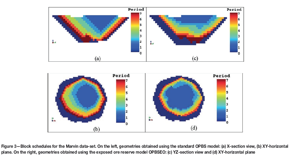
The pits obtained when scheduling the Marvin case are presented in Figure 3, showing a YZ-section view and a horizontal plane for both schedules, obtained from OPBS (left) and OPBSEO (right). The colours correspond to the periods at which the blocks are extracted.
First of all, there is a large difference between the extraction geometries; it is worth noting that for this case, the pits obtained using the OPBSEO model are more operational than those obtained using OPBS.
Both models aim to maximize NPV and therefore to extract blocks with higher grades as soon as possible, but OPBSEO must ensure a minimum exposed ore reserve at the beginning of each period, allowing a large horizontal surface in the bottom of each pit.
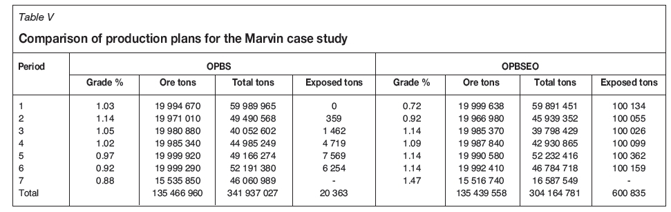
Production plans obtained from models OPBS and OPBSEO are shown in Table V, where the impact of the exposed ore reserve constraints appears in terms of ore and total tonnages, grade profile over time, and exposed tonnage (as metal) per period, as in Table III. It is interesting to observe that there are no differences in terms of ore tonnage, but the OPBSEO model reported 11% less total tonnage than the solution obtained using the OPBS model (recall that in this case the model must ensure at least 4 months' supply of exposed ore at the beginning of each period), but about the same amount of ore (the difference is less than 0.1%).
Table VI shows the discounted values for both models. The results are similar to the other example: OPBS is able to provide a schedule with higher value by extracting high-grade blocks as soon as possible, while OPBSEO delays some of these blocks to ensure minimum exposed ore reserves in order to keep ore available for future exposure. The difference in NPVs in this case is about 5%, but we observe that the solutions are optimal only within the time horizon considered here. Indeed, the production plans suggest that additional periods may lead to different solutions and higher NPVs.

Conclusions and open questions
In this paper, the concept of exposed ore reserve is introduced in a mathematical model and defined at a given period as the set of blocks for which all its preceding blocks have been already extracted, but not the block itself. A new integer programming model, named OPBSEO, to generate block schedules under exposed ore reserve requirements has been presented and tested in a set of standard instances.
First, the model was tested on a two-dimensional instance to validate the solutions that it provided, with satisfactory results. The model was then tested on two realistic instances, providing comparisons between the solutions from the OPBSEO model and the equivalent one, but without exposed ore requirement, named OPBS. The solutions obtained with the aid of the proposed model are consistent with those obtained by other optimization models for mine planning that do not have exposed ore reserve requirements in their formulation.
The new model, compared with similar optimization models without the exposed ore reserve requirement, suffers from a small reduction in the value of the solution due to the additional requirements included. However, the geometrical nature of the new solutions obtained in the tests performed exhibits better operational spaces and regularity. While it is not possible to generalize this property of the solutions to other instances, it is believed that the model has the potential to produce results that are better suited to the type of operational spacing needed in mining operations, thus adding a valuable alternative to the current tools used by mine planners. Besides, this new requirement ensures the quantity of metal produced from the beginning of each period in the schedule, making compliance with medium- and short-term mine planning stages easier.
A potential research path to pursue in the future relates to the definition of the exposed ore reserve. In the present version we only consider a minimum amount of metal readily available at the beginning of every period, but other metal components could also be considered, expressed in terms of tonnage, grades, or economic value; or this requirement could be relaxed, for example, to consider blocks at a maximum distance from surface that is larger than only one bench. Other important questions for future study relate to assessing the suitability of the model for different types of deposits and mining operations, and which conditions are required in order to produce solutions with the geometrical properties that have been observed in the present study.
The proposed model exhibits great potential in terms of applicability, but further algorithmic research is required to improve the computational execution time in the case of very large instances. However, it is important to mention here that the present paper has focused on introducing the concept and presenting the associated model. As the results obtained in the instances tested are encouraging enough to warrant additional research, it is believed that the first step taken in this study will serve as a solid foundation for new ways of thinking about mine planning, to the benefit of industry and practitioners.
Acknowledgments
This research has been partially supported by FONDECYT Program, Grant-1130816; Basal Project CMM-Centro de Modelamiento Matemático, Universidad de Chile; and Basal Project FB0809 AMTC-Advanced Mining Technology Center, Universidad de Chile.
References
Amankwah, H., Larsson, T. and Textorius, B. 2014. A maximum flow formulation of a multi-period open-pit mining problem. Operational Research, vol. 14, no. 1. pp. 1-10. [ Links ]
Bienstock, D. and Zuckerberg, M. 2010. Solving LP relaxations of large-scale precedence constrained problems. Operational Research, vol. 14. pp. 1-14. [ Links ]
Bley, A., Boland, N., Fricke, C., and Froyland, G. 2010. A strengthened formulation and cutting planes for the open-pit mine production scheduling problem. Computers and Operations Research, vol. 37, no. 9. pp.1641-1647. [ Links ]
Boland, N., Dumitrescu, I., Froyland, G., and Gleixner, A. 2009. LP-based disaggregation approaches to solving the open-pit mining production scheduling problem with block processing selectivity. Computers and Operations Research, vol. 36, no. 4. pp. 1064-1089. [ Links ]
Caccetta, L. 2007. Application of optimisation techniques in open-pit mining. Handbook of Operations Research in Natural Resources. Weintraub A., Romero, C., Bjorndal, T., and Epstein, R. (eds.). Springer, New York. [ Links ]
Caccetta, L. and Hill, S. 2003. An application of branch and cut to open-pit mine scheduling. Journal of Global Optimization, vol. 27. pp. 349-365. [ Links ]
Chicoisne, R., Espinoza, D., Goycoolea, M., Moreno, E., and Rubio. E. 2012. A new algorithm for the open-pit mine production scheduling problem. Operations Research, vol. 60, no. 3. pp. 517-528. [ Links ]
Cullenbine, C., Wood, R.K., and Newman, A. 2011. A sliding time window heuristic for open-pit mine block sequencing. Optimization Letters, vol. 5, no. 3. pp. 365-377. [ Links ]
Dagdelen, K. and Johnson, T. 1986. Optimum open-pit mine production scheduling by lagrangian parameterization. Proceedings of the 19th International Symposium on Application of Computers and Operations Research in the Mineral Industry (APCOM). Ramani, R.V. (ed.). SME, Littleton, CO. pp. 127-141, [ Links ]
Dagdelen, K. and Akaike, A. 1999. A strategic production scheduling method for an open-pit mine. Proceedings of the 28th International Symposium on Application of Computers and Operations Research in the Mineral Industry (APCOM). Proud, J., Dardano, C., and Francisco, M. (eds.). SME, Littleton, CO. pp. 729-738. [ Links ]
Espinoza, D., Goycoolea, M., Moreno, E., and Newman, A. 2013. Minelib: a library of open-pit mining problems. Annals of Operations Research, vol. 206, no. 1. pp. 93-114. [ Links ]
Fricke, C. 2006. Applications of integer programming in open-pit mining. PhD thesis, Department of Mathematics and statistics, university of Melbourne, Melbourne. [ Links ]
Gaupp, M. 2008. Methods for improving the tractability of the block sequencing problem for open-pit mining. PhD thesis, Colorado school of Mines, Golden, Co. [ Links ]
Hochbaum, D. and Chen, A. 2000. Performance analysis and best implementation of old and new algorithms for the open-pit mining problem. Operations Research, vol. 48. pp. 894-914. [ Links ]
Hustrulid, W. and Kuchta, K. 2006. Open-Pit Mine Planning and Design (2nd edn). Taylor and Francis, London. [ Links ]
Jélvez, E., Morales, N., Nancel-Penard, P., Peypouquet, J., and Reyes, P. 2016. Aggregation heuristic tor the open-pit block scheduling problem. European Journal of Operational Research, vol. 49, no. 3, pp. 1169-1177. [ Links ]
Johnson, T.B. 1968. Optimum open-pit mine production scheduling. PhD thesis, Operations Research Department, University of California, Berkeley. [ Links ]
Johnson, T.B. 1969. Optimum open-pit production scheduling. A Decade of Digital Computing in the Mineral Industry. Weiss, A. (ed.). AIME, New York. pp. 539-562. [ Links ]
Lambert, W.B. and Newman, A. 2013. Tailored lagrangian relaxation for the open.pit block sequencing problem. Annals of Operations Research, vol. 222, no. 1. pp. 1-20. [ Links ]
Lerchs, H. and Grossmann, 1.1965. Optimum design for open pit mines. CIM Bulletin, vol. 58. pp. 47-54. [ Links ]
Mitchell, S. 2009. An introduction to pulp for Python programmers. The Python Papers Monograph, vol. 1. [ Links ]
Picard, J. 1976. Maximal closure of a graph and applications to combinatorial problems. Management Science, vol. 22, no. 11. pp. 1268-1272. [ Links ]
Ramazan, S., Dagdelen, K., and Johnson, T. 2005. Fundamental tree algorithm in optimizing production scheduling for open-pit mine design. Mining Technology, vol. 114, no. 1. pp. 45-54. [ Links ]
Tabesh, M. and Askari-Nasab, H. 2011. Two-stage clustering algorithm for block aggregation in open pit mines. Mining Technology, vol. 120, no. 3. pp. 158-169. [ Links ]
Zhang, M. 2006. Combining genetic algorithms and topological sort to optimize open-pit mine plans. Proceedings of the 15th International Symposium on Mine Planning and Equipment Selection (MPES). Cardu, M., Ciccu, R., Lovera, E., and Michelotti, E. (eds.). FIORDO S.r.l. Torino, Italy. pp. 1234-1239. [ Links ]
Paper received Jun. 2014
Revised paper received Oct. 2015.
The Southern African Institute of Mining and Metallurgy, 2016. ISSN 2225-6253

