PAPERS - DANIE KRIGE GEOSTATICAL CONFERENCE

 

When should uniform conditioning be applied?

 

 

K. Hansmann

University of the Witwatersrand, Johannesburg, South Africa

 

 

---

SYNOPSIS

Blindly applying any methodology to estimate the recoverable resources of a mineral deposit without considering the suitability of the approach to the deposit being evaluated can render misleading results. While 'running the software' provides an answer, one should, amongst numerous other considerations, understand the impact the underlying distributions and assumptions have on the validity of the result.
Uniform conditioning (UC) is a nonlinear estimation method that models the conditional distribution of smallest mining unit (SMU) block grades within panels, and localized uniform conditioning (LUC) places these SMU at plausible locations within a panel. The localization process does not improve the accuracy of the UC result, but rather presents the result in a more practical format; particularly for use in mine planning.
A case study was carried out to compare the suitability of UC and LUC on two hypothetical data-sets. The data-sets are simulated realizations of a normal grade distribution and a highly skewed lognormal grade distribution which are akin to grade distributions found in mineral deposits. The estimation methods were applied to both data-sets, and the results compared with the actual grades of the simulated realizations. This paper presents an overview of UC and LUC, with discussions around the case study results.

Keywords: change of support, Gaussian anamorphosis, localized uniform conditioning, lognormal distribution, normal distribution, uniform conditioning

---

 

 

Introduction

Uniform conditioning (UC) is a nonlinear estimation technique that estimates the conditional distribution of metal and tonnage above cut-off within a mining panel. It does not directly estimate grade, although grade is a typical outcome from the estimated metal-tonnage distribution or the results produced by localized uniform conditioning (LUC). UC results are typically presented as a recoverable resource above multiple cut-off grades. The advantage of UC is that it can be used on widely spaced data, across domains that are not strictly stationary, provided that there is sufficient data for a conditionally unbiased estimate of the panel mean grade (Rivoirard, 1994).

Previous studies where UC has been applied to porphyry copper deposits (Deraisme et al., 2008; Deraisme and Assibey-Bonsu, 2011; Millad and Zammit, 2014) show the application of the method to normal grade

distributions. Additional studies have applied this approach to gold deposits (Assibey-Bonsu, 1998; Humphreys, 1998) and an iron ore deposit (De-Vitry et al., 2007), indicating that the method is applicable on skew, lognormal distributions. While UC has been practically applied to different types of deposit, it is not known how well UC predicts actual grades for the underlying grade distribution.

This paper discusses the UC estimation method as well as the popular add-on, LUC, presented by Abzalov (2006). A case study is presented that compares UC and LUC estimates of two hypothetical data-sets, referred to herein as scenario 1 and scenario 2. Scenario 1 is a normally distributed grade distribution and scenario 2 is a skew, lognormally distributed grade distribution, both of which are compared against the simulated realizations that represent the actual grades.

The conditions found in the two data-sets are similar to those found in naturally occurring mineral deposits. The aim of this investigation is to determine the underlying conditions of the grade distribution that produces favourable results when applying UC, and subsequently LUC, to such data-sets.

 

Uniform conditioning workflow

The following section describes a UC with LUC workflow, which follows the process outlined in Figure 1.

 

 

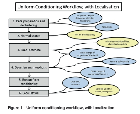
Data preparation and declustering

This initial part of the UC workflow is to prepare and carry out exploratory data analyses, including histograms, to understand the sample grade distribution and variability in the deposit. The data must be appropriately declustered, so that the normal score transforms of the grades are an accurate representation of the grade distribution. This is important for the Gaussian anamorphosis function (to be discussed later), and failure to correctly complete this will affect the results of the UC estimate.

Normal scores

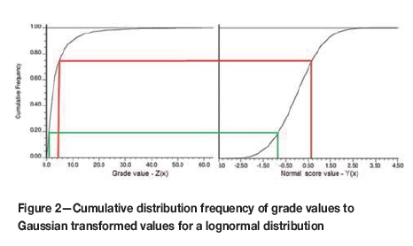
As the discrete Gaussian model (DGM) for change of support is used for UC, the data must be transformed to the equivalent Gaussian (or normal score) values using declustered weights. This is performed by transforming the cumulative distribution frequency (CDF) of the original grades to a Gaussian probability CDF, on a percentile to percentile basis for the entire data-set. Figure 2 shows the CDF of a lognormal grade distribution (data from scenario 2) on the left, with the green and red lines showing percentile paired mapping of values to the equivalent normal score values on the right.

 

 

The DGM relies upon the assumption of bivariate Gaussianity of the transformed grades (Rivoirard, 1994). Bivariate Gaussianity means that any linear combination of the Gaussian transformed data is also Gaussian. Several tests exist to determine if the transformed data conforms to such conditions, and is therefore suitable for use with the DGM. Schofield (1988), Rivoirard (1994) and Humphreys (1998) give practical examples on how these tests may be run.

Panel estimates

The quality of the panel estimate determines the success of the UC estimation (Rivoirard, 1994). A panel estimate should be conditionally unbiased (Rivoirard, 1994; De-Vitry et al., 2007), so that the UC conditional grade distribution will be an accurate estimate of the actual grade distribution. The panel estimate can be carried out using any linear estimator, but conventionally ordinary kriging (OK) is used.

The panel size should be chosen relative to the spacing of the sample data. De Vitry et al. (2007) suggested that the panel should be as small as possible to ensure an accurate estimate, but large enough for minimal conditional bias of the estimate. The number of smallest mining units (SMU) within the panel is linked to the resolution of the grade-tonnage relationship, as the number of SMU discretizes the grade-tonnage curve of the panel (Harley and Assibey-Bonsu,2007).

Gaussian anamorphosis

The DGM can be used to derive the marginal histograms at different supports. The Gaussian anamorphosis function is modelled by a set of Hermite polynomials, weighted with an accompanying set of Hermite coefficients. A full description of Hermite polynomials and how these may be calculated is given by Rivoirard (1994).

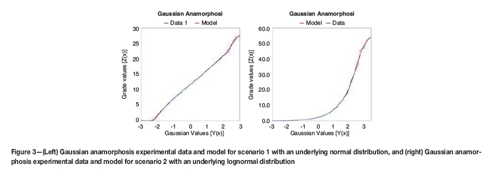
A point and fitted model anamorphosis function for a normal and lognormal distribution are shown in Figure 3. The anamorphosis function for the lognormal distribution is constructed from the normal score data, by plotting pairs of grade and Gaussian transformed grade values.

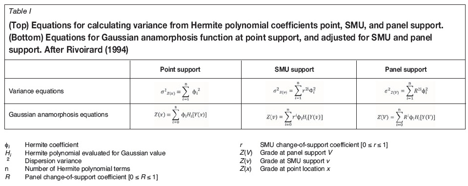
The Hermite polynomials are functions of the standard Gaussian distribution, and therefore they express probabilities and have the properties of a standard Gaussian distribution (data is symmetrically distributed around the mean value of zero, and has a unit variance). An additional property (see Table I) shows the variance of the grade Z(x) expressed by the sum of Hermite coefficients, excluding the 0th, which describes the mean.

The number of Hermite coefficients used to fit the anamorphosis model can vary, and the optimal number depends on the how well the polynomial set fits the underlying distribution. Neufeld (2005) recommends using less than 100 coefficients, although 20 to 30 coefficients are usually sufficient.

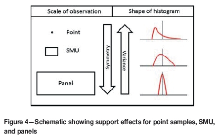
The variance of grades depends on the support that the grade represents, and a change-of-support model, like the DGM, is used to predict the distribution of grade at different supports. Grades at a point support have a higher variance than grades of SMU, which similarly have a higher variance than grades of panels. As the support of a grade increases, so the grade values tend towards the population mean, have less deviation from it, and are more symmetrical around it (Figure 4).

 

 

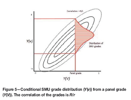
There is a correlation between the distribution of grades seen at a point support and the distribution of grades seen at a SMU support, named the SMU change-of-support coefficient (r). Similarly, there is a correlation between the distribution of grades seen at a point support and the distribution of grades seen at a panel support, named the panel change-of-support coefficients (R). The ratio R/r is the correlation of SMU grades and panel grades. The R and r change-of-support coefficients are determined by solving the variance equations and the Gaussian anamorphosis equations at SMU and panel supports, shown in Table I (Rivoirard, 1994).

Uniform conditioning

The schematic in Figure 5 shows the relationship between grades at a SMU support, grades at panel support, and how a distribution of SMU grades is conditional on panel grade. A low R/r ratio indicates a weak correlation between the SMU and panel grades, which is caused by a high-nugget semivar-iogram and/or short semivariogram ranges relative to the data spacing. A high R/r ratio is indicative of a strong correlation between SMU and panel grades, which indicates good grade continuity in the deposit.

 

 

Localization

The result of a UC estimate is presented as a distribution of grades, shown as metal content and tonnages reported for a series of cut-off grades. While this is insightful information about the grade-tonnage distribution, it is not a particularly practical data format as the SMU location is not provided.

Abzalov (2006) presents LUC as a simple extension to UC that provides a practical solution for visualizing grades at the SMU level. A UC grade-tonnage distribution is decomposed to a series of grade values that reproduce the grade-tonnage relationships. These plausible SMU grades are located into a SMU model based on the rank location of grades from a linear estimate of equally sized blocks. This results in a direct grade model at the SMU resolution that respects the grade-tonnage distributions of the UC panels and attempts to reflect the localized spatial grade distribution within the panel.

Case study

The objective of this case study is to assess the suitability of UC and LUC for two data-sets with different grade distributions, namely scenario 1 and scenario 2. The two scenarios are distinctly different and represent two end-members of the range of grade distributions that may typically be seen in mineral occurrences, being a symmetrical distribution and a positively skewed distribution. The grade distributions were synthetically generated and sampled to mimic how this would be done in a mineral exploration project.

The UC with localization procedure described in this paper was followed for both data-sets, as outlined in Figure 1.

Description of case study data

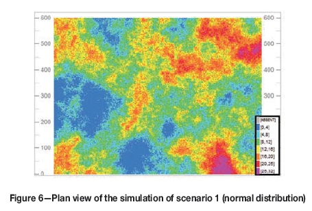
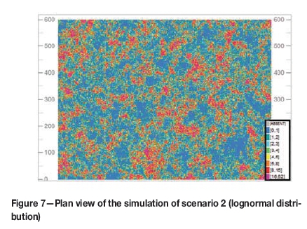
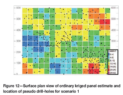
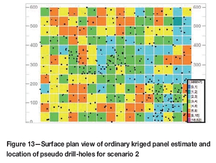
Two sets of simulated data were generated, which were used as base data for the assessment. A single realization was simulated on a 2 m x 2 m x 2 m point grid, over a 800 m x 600 m area, with a thickness of 200 m, for each distribution. A plan view at surface through both simulations is shown in Figure 6 and Figure 7.

 

 

 

 

Statistics and variography

A spatially representative subset of data was taken from both simulations, which makes up the sample database used for this project. A total of 417 pseudo drill-holes, each containing 100 composites, was taken over the study area. The area is densely sampled, and this drilling grid would be consistent with that of a feasibility-stage project.

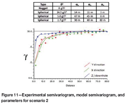
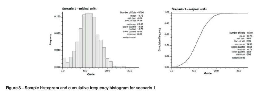
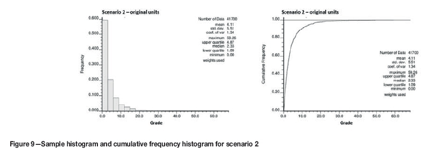
Although both scenarios are equally sampled (at a density of 1%), the drill-hole spacing relative to the semivar-iogram ranges for scenario 1 is closer than for scenario 2. For scenario 1, the samples are spaced at approximately one-third of the semivariogram ranges (120 m) in X and Y, while for scenario 2 the samples are spaced at approximately the maximum semivariogram range (40 m). Statistics of both scenarios are compared, but there is no correlation between them as the simulations were run independently. Declustered statistics are presented in Table II, histograms in Figure 8 and Figure 9, and modelled semivariograms in Figure 10 and Figure 11.

 

 

 

 

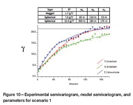
In scenario 1, the grade distribution is symmetrical, with a comparatively low nugget effect (12%) and well-defined continuity up to distances of 170-300 m. Slight anisotropy was evident, and possibly some zonal anisotropy seen in the Y-direction where the variance does not reach the sill value. The distribution is approximately normal, and is similar to what one would find in a porphyry copper mineral occurrence. The first distribution has a smaller range of grade values than the second (approximately half).

In scenario 2, the grade distribution is approximately lognormal, supported by the shape of the histogram. This distribution has the characteristics of being asymmetrical, strongly positively skewed, with a long tail. There is a higher nugget effect (26%), with long-range continuity of approximately 60-90 m. The coefficient of variation (CoV) for scenario 2 is higher (1.3) than that of scenario 1 (0.4), showing a wider spread and higher variability of grade values.

Panel estimates

Panel grade estimates, using OK, were produced for both scenarios with the intent of minimizing conditional bias while retaining some local variability. The block sizes were chosen relative to the average sample spacing, at 50 m χ 50 m χ 20 m. Ten discretization points were chosen in the X and Y directions, based on a quantitative kriging neighbourhood analysis (QKNA) optimization of the block variance. Discretization points in the Z direction were chosen to be equal to the compositing length. A sufficiently large search neighbourhood was chosen for the panel estimate to ensure high slopes of regression, without the introduction of too many (>5%) negative kriging weights.

The panel model estimation for scenario 1 had a mean slope of regression of 0.97; while that of the scenario 2 panel model estimation was 0.72. Figure 12 and Figure 13 show plan views of the respective scenarios, at surface elevation. Comparing these to the simulated data (Figure 6 and Figure 7), the grade smoothing effect and reduction of variance from the OK is evident.

 

 

 

 

Change of support

Sample data was converted to normal scores and tested for bivariate Gaussianity. For both scenarios, the test results were consistent with bivariate Gaussian conditions of the Gaussian transformed data. Change of support was carried out for each scenario using the DGM, with parameters shown in Figure 3.

In scenario 1 the SMU change-of-support coefficient indicates a strong correlation between point and SMU grades. For scenario 2, the SMU change-of-support coefficient implies a weak correlation between point and SMU grades and is a result of the high nugget effect.

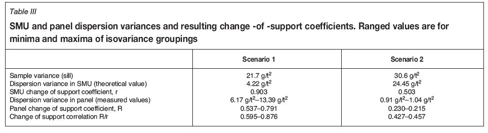
Panel change-of-support coefficients are measured from the direct variance of estimated panel grades. Well-informed panels, as defined by the number of samples in the neighbourhood and semivariogram ranges, will have better estimation confidence. To account for this, different panel change-of-support correlations are used for panels with similar confidence in the estimation. Three such isovariance groupings were used for each scenario, and the ranges of these results are shown in Table III. Relatively higher variances of estimated panel grade groupings are typically from better-informed areas where there is better grade continuity that results in a greater spread of estimated panel grades. Conversely, relatively lower estimated panel grade variance groupings are for worse-informed areas, where there is more evidence of smoothing and panel estimates are closer to the mean, giving rise to less variance

Running uniform conditioning and localization

UC was carried out for both data-sets using the panel model and DGM. After completion of UC, the model was localized using a local SMU model, which was estimated using smaller kriging neighbourhoods to reflect local variability.

 

Discussion on uniform conditioning

The performance of UC may be assessed by how closely the UC grade-tonnage estimate conforms to the actual simulated model and an OK model, as a benchmark for a linear estimator. This comparison was made globally, to demonstrate the effects of incorrectly predicting the extractable tonnage of the deposit, and locally, to demonstrate the effects of getting individual panel grades right/wrong.

Global grade-tonnage assessment

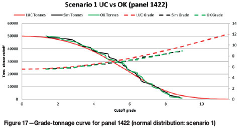
The grade-tonnage relationship for the normally distributed scenario is shown in Figure 14. The global UC prediction of tons and grades is very close to the actual grades, and shows a slight improvement on the OK grade-tonnage curve.

 

 

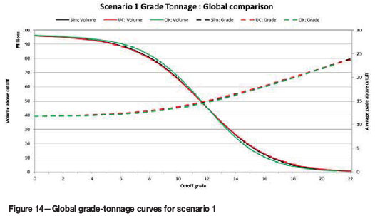
In the case of the normally distributed grades (scenario 1), where there is good data coverage (relative to the semivariogram ranges), OK performs well for determining recoverable resources. Slopes of regression for the OK model were, on average, close to unity, indicating a very low conditional bias (which is reflected in the OK estimates being close to the actual values). However, UC marginally outperforms OK in terms of estimating a recoverable resource, as it more closely predicts the grade and tonnage of the simulated reality. For low cut-off grades, there is slightly less tonnage than predicted for the both the OK and UC model, but the UC estimates are closer to the actual values.

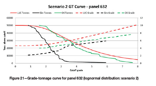
Where the grade data has an underlying lognormal distribution (scenario 2) with relatively poor data coverage, the simulated model shows a decline in tonnage (or volume) as the cut-off grade increases (Figure 15). OK generates a moderate estimation of the grade and tonnage extractable for any cut-off grade. This lack of adherence to the grade-tonnage curve can be explained by a grade smoothing, which was expected, as the slopes of regression of the panel estimate were, on average, poor. UC gives a better result than OK, but the resultant estimation of grades and tonnage does not closely conform to the actual values. As the selectivity increases (i.e. high-grade areas are targeted), the average grade of the actual material will be higher than the OK model predicts.

 

 

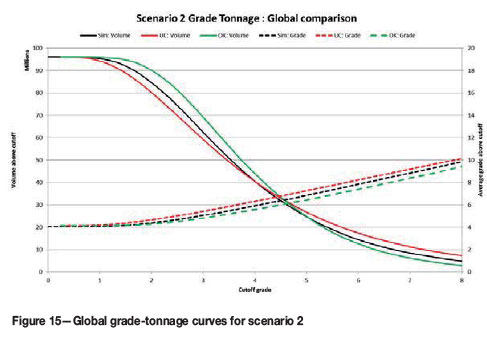
At low cut-off grades, a linear estimated model frequently shows an overestimation of volume or payable ground. This is referred to as the 'vanishing tons' problem as described by David (1977), which is seen when mining commences and less material is recovered than was predicted. This is caused by a conditional bias and/or smoothing in the estimate, which are reflected respectively by low slopes of regression and/or higher estimation variance in the estimated result. This phenomenon is amplified by a high nugget effect and small block sizes used for estimation.

In order to resolve a conditional bias, one can estimate grades into larger blocks. However, estimating into larger blocks can produce an over-smoothed histogram, or too much average material, and does not provide the accuracy required to select blocks for mining. This is the 'kriging oxymoron' (Isaaks, 2004), which states that a kriged estimate cannot be conditionally unbiased and accurate at the same time. UC uses the 'conditionally unbiased' large block estimator to condition the average of a distribution of small blocks, thereby maintaining the correct grade-tonnage curves and applying a conditional distribution to obtain an accurate histogram of small block (SMU) grades. This attempts to satisfy the apparent contradiction embodied in the kriging oxymoron.

Local grade-tonnage assessment

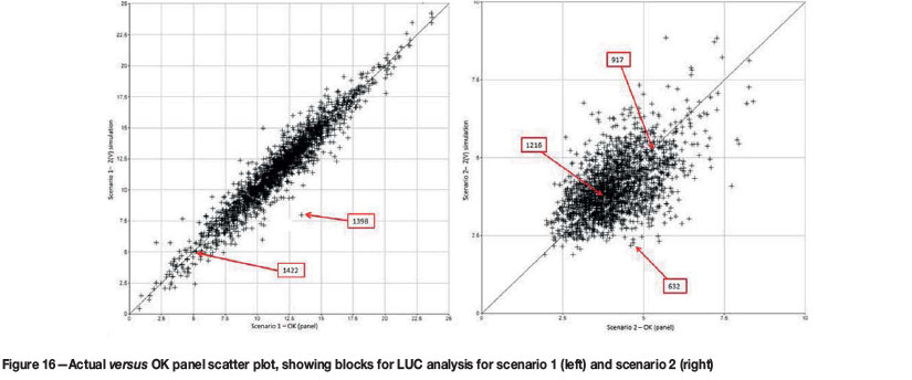
An assessment was done to compare the grade-tonnage results of panels that are well estimated and did not contain a conditional bias (as determined by the slope of regression) against poorly estimated panels. Panels chosen for this assessment are shown in Figure 16, where values with the better slopes of regression fall on or close to the 1:1 regression line.

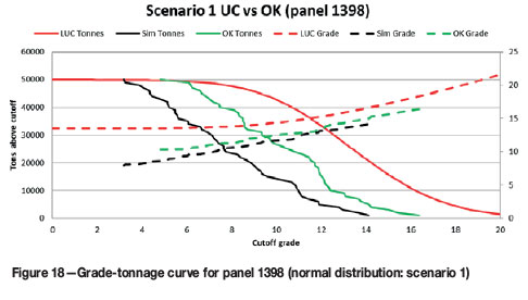
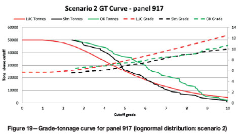
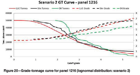
For the normally distributed data, if the mean panel grade estimate is correct, the UC accurately predicts the distribution of grades and tonnage (Figure 17). For the lognormally distributed data, UC predicts the grade-tonnage relationship (Figure 19 and Figure 20) fairly well. For both distributions, if the mean panel grade is wrong, the distribution of SMU grades will not necessarily match the simulated distribution (Figure 18 and Figure 21). It appears that, in addition to an unbiased panel estimate, UC performs slightly better on an individual panel basis when the underlying distribution is normal.

 

 

 

 

 

 

 

 

 

 

Localization ranking assessment

The localization of the UC result places individual SMU grades (derived from the SMU grade-tonnage curve within the panel) at specific locations within the panel, based on the estimated grades of the OK SMU model. The success of the localization is verified by visual comparison and by statistically comparing the rank values of the actual versus the UC ranking (Figure 22).

 

 

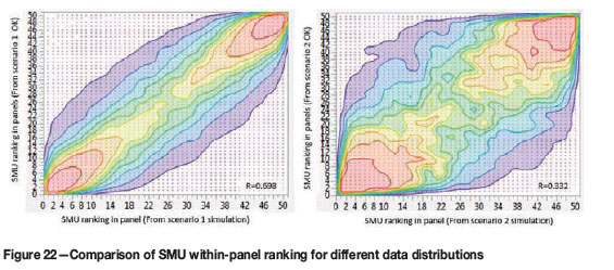
The success of localization depends entirely on the reliability of the OK SMU estimate. However, the smoothing and inaccuracy of this estimate is the prime motivation to use UC in preference to linear estimates. If the OK SMU estimate provides a good spatial representation of the local grades, then the location of the UC grades within the panel will be more accurate. This confirms Abzalov's (2006) findings that the localization success is dependent on available data (among other factors).

If the data is closely spaced enough to provide accurate localization, then it is also likely that the data is sufficiently closely spaced for a linear estimation to accurately predict the model grade value. In this circumstance, the benefit of using a nonlinear UC estimator over a linear estimator is not as significant as the benefit seen with widely spaced data. This is evident in the grade-tonnage predictions for the well-estimated data, where the OK and UC results are similar; and the predictions for the poorly estimated data, where the UC results show a significant improvement over the OK results.

Although LUC is a useful addition to UC, it does not improve the accuracy of the UC estimate and the localization algorithm cannot predict the placements of SMU beyond the available data. This is the main problem: one cannot simultaneously know the local mean and the local variability from limited local data. The single largest contribution of the localization approach is to present a UC model in a more accessible and immediately useful format for mine planning.

 

Conclusions

UC performs well in terms of estimating grades and tonnages when there is a normal underlying grade distribution and good sample coverage relative to the variogram ranges, which result in low conditional biases. In such circumstances a linear estimator can also closely predict recoverable resources and provide a spatially representative grade model, although the UC estimate of tons and grades is slightly better.

When there is an underlying lognormal distribution and poor sample coverage relative to variogram ranges, conditional biases of a linear panel estimate will occur. This results in UC providing a more accurate global estimate of grades and tonnage than a linear estimate. The individual panel results predict the actual grade and tonnage distribution when there is no evidence for conditional bias for that panel.

LUC results are favourable when there is sufficient closely spaced data, in which case it is likely that a linear estimation could also accurately predict the model grade values. Therefore, the benefit of using a nonlinear UC estimator over a linear estimator is more significant when the data is widely spaced.

 

Acknowledgments

My thanks to those who reviewed this work, and particularly to Michael Harley of Anglo American for his advice.

 

References

Abzalov, M.Z. 2006. Localised uniform conditioning (LUC): a new approach for direct block modelling. Mathematical Geology, vol. 38, no. 4. pp. 393-411.         [ Links ]

Assibey-Bonsu W. 1998. Use of uniform conditioning technique for recoverable resource/reserve estimation in a gold deposit. Proceedings of Geocongress 1998. Geological Society of South Africa, Johannesburg. pp. 68-74.         [ Links ]

David, M. 1977. Geostatistical Ore Reserve Estimation (4th impression). Elsevier, New York. pp. 301-320.         [ Links ]

De-Vitry, C., Vann, J., and Arvidson, H. 2007. A guide to selecting the optimal method of resource estimation for multivariate iron deposits. Proceedings of Iron Ore2007, Perth, Australia. Australasian Institute of Mining and Metallurgy, Melbourne. pp. 67-77.         [ Links ]

Deraisme, J. and Assibey-Bonsu, W. 2011. Localised uniform conditioning in the multivariate case - An application to a porphyry copper gold deposit. Proceedings of the 35th International Symposium on Application of Computers and Operations Research in the Minerals Industry (APCOM), Wollongong, Australia, 24-30 September 2011. Baafi, E.Y., Kininmonth, R.J., and Porter, I. (eds.). Australasian Institute of Mining and Metallurgy, Melbourne.         [ Links ]

Deraisme, J., Rivoirard, J., and Carrasco Castelli, P. 2008. Multivariate uniform conditioning and block simulations with discrete gaussian model: Application to the Chuquicamata deposit, Proceedings of the VIII International Geostatistics Congress (Geostats2008), Santiago, Chile, 1-5 December 2008. Gecamin, Santiago. pp. 69-78.         [ Links ]

Harley, M. and Assibey-Bonsu, W. 2007. Localised uniform conditioning: How good are the local estimates? Proceedings of the 33rd International Symposium on Application of Computers and Operations Research in the Minerals Industry (APCOM), Santiago, Chile, 24-27 April 2007. Magri, E.J. (ed.). Gecamin, Santiago. pp. 105-112.         [ Links ]

Humphreys, M. 1998. Local recoverable estimation: A case study in uniform conditioning on the Wandoo Project for Boddington Gold Mine. Proceedings of a One-day Symposium: Beyond Ordinary Kriging, Perth, 30 October 1998. Geostatistical Association of Australia. pp. 63-75.         [ Links ]

Isaaks, E. 2004. The kriging oxymoron: A conditionally unbiased and accurate predictor (2nd edn.). Proceedings of Geostatistics Banff2004. Leuangthong, O. and Deutsch, C.V. (eds). Springer. pp. 363-374.         [ Links ]

Neufeld, C.T. 2005. Guide to recoverable reserves with uniform conditioning. Guidebook Series, volume 4. Centre for Computational Geostatistics (CCG), University of Alberta, Canada.         [ Links ]

Millad, M.G. and Zammit, K.M. 2014. Implementation of localised uniform conditioning for recoverable resource estimation at the Kipoi Copper Project, DRC. Proceedings of the Ninth International Mining Geology Conference. Australasian Institute of Mining and Metallurgy, Melnourne. pp. 207-214.         [ Links ]

Rivoirard, J. 1994. Introduction to Disjunctive Kriging and Nonlinear Geostatistics. Centre de Geostatistique, Ecole des Mines, Paris, France.         [ Links ]

Schofield, N. 1988. Ore reserve estimation at the Enterprise gold mine, Pine Creek, Northern Territory, Australia. Part 1: structural and variogram analysis. CIM Bulletin, vol. 81, no. 909. pp. 56-66.         [ Links ]

Verly, G. 1986. Multigaussian kriging - a complete case study. Proceedings of the 19 th International Symposium on Application of Computers and Operations Research in the Minerals Industry (APCOM), Littleton, CO. Ramani, R.V. (ed.). Society of Mining Engineers, Littleton, CO. pp. 283-298.         [ Links ]

 

 

This paper was first presented at, The Danie Krige Geostatistical Conference 2015, 19-20 August 2015, Crown Plaza, Rosebank.