PAPERS - DANIE KRIGE GEOSTATICAL CONFERENCE

 

Resource estimation for deep tabular orebodies the AngloGold Ashanti way

 

 

T. Flitton; R. Peattie

AngloGold Ashanti

 

 

---

SYNOPSIS

The extreme depths and consequent expense of drilling and sampling the gold-bearing reefs of the Witwatersrand Basin have resulted in limited data being available for estimation of grade ahead of the mining face. There is, however, a wealth of information from mined-out areas of these deposits. This estimation challenge resulted in the development of a unique method of Mineral Resource estimation.
AngloGold Ashanti (AGA) utilizes a technique termed macro cokriging (MCK), which allows for the integration of the limited advanced borehole data with the large chip sample data-sets from the previously mined-out areas by adopting a Bayesian geostatistical approach. The MCK process, in short, is the estimation of mixed support size data together with the application of four-parameter distribution models.
The gold value estimation for the Carbon Leader Reef (CLR) on the AGA TauTona Mine is used in this paper as a case study of the process and to demonstrate the effectiveness of this technique through production reconciliation. The current method has been proven over the last 20 years and is now an established part of the Mineral Resource evaluation process within AGA.

Keywords: resource evaluation, Bayesian assumption, macro cokriging, mixed support, four-parameter distribution

---

 

 

Introduction

Owing to the extreme depths of the gold-bearing reefs at the AngloGold Ashanti (AGA) Witwatersrand operations and the prohibitive expense and time involved in drilling boreholes to the required depth, only limited drilling and sampling data is available ahead of the mining face. Whereas traditional estimation techniques are interpolative, within the Witwatersrand the estimation is primarily extrapolative, with the majority of the data being sourced from the mined-out areas. This significant challenge to estimation resulted in the development of a unique method of Mineral Resource estimation and evaluation.

 

The process

Macro cokriging (MCK) was first introduced in 1994 and has been is use for 20 years by AGA. There are three key aspects to this technique; namely a Bayesian approach to estimation, the estimation of mixed support size data (MCK), and the utilization of four-parameter distributional models.

(1) The Bayesian process followed allows for the integration of the limited advanced data with the large data-set from the previously mined-out areas. Krige et al. (1990), and later Dohm (1995), proposed the use of a Bayesian geostatistical approach where 'the geological, statistical and spatial characteristics observed in the known population area holdfor the virgin areas'

(2) Estimation by MCK of two different sampling support sizes, one at block support, representing the dense underground chip sampling data and the other cluster support, representing the widely spaced borehole data (Dohm, 1995; Chamberlain, 1997). The MCK technique is not strictly cokriging, but the modification of the diagonal kriging matrix to reflect different nugget effects related to different data supports. The methodology also assumes the same spatial covariance structure for the different data supports and thus does not use cross-variograms

(3) The continued development of distributional models beyond the use of the two- and three-parameter lognormal models led to the development of four-parameter distributional models by Sichel (1990) and Sichel et al. (1992) that are more applicable for the gold reefs of the Witwatersrand. Estimation is done in natural logarithmic (Ln) space because of the highly skewed gold distribution. The final gold estimates are calculated by back-transforming the estimates using four-parameter distribution models (Dohm, 1995; Chamberlain, 1997).

Many of the processes developed and used by AGA are based on the work completed and detailed by Dohm (1995) and Chamberlain (1997).

The unique estimation method followed does not, however, detract from the criticality of having a sound geological model. It is imperative for this and any other estimation process that the geological model accurately represents the understanding of the deposit.

Location and data

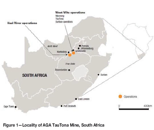
AGA's TauTona Mine lies on the West Wits Line, just south of Carletonville in North West Province, about 70 km southwest of Johannesburg (Figure 1). Mining at this operation commenced over 50 years ago and currently takes place at depths ranging from 2000 m to 3640 m below surface. The mine has a three-shaft system and employs a sequential and/or scattered grid mining method to extract the gold in the deep, narrow, tabular orebody. The grid is pre-developed through a series of haulages and crosscuts. Stoping takes place by means of breast mining using conventional drill-and-blast techniques. The smallest mining unit (SMU) is 100 m χ 100 m.

 

 

The CLR is the principal economic horizon at TauTona. The CLR is located near the base of the Johannesburg Subgroup, which forms part of the Central Rand Group of the Witwatersrand Supergroup. The CLR is a thin (on average 20 cm thick) tabular, auriferous quartz pebble conglomerate.

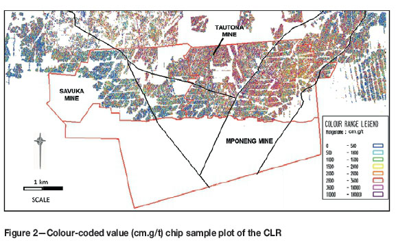
The sampling data is comprised of underground chip sample sections (425 917 points), underground boreholes, and surface boreholes from TauTona and neighbouring mines. Underground sampling is in the form of chip sampling taken on the mining face using a hammer and chisel. All sample locations are reported as a composite over a mineralized width, resulting in a single channel width (cm) and gold metal accumulation value (cm.g/t) (Figure 2). The natural logarithms (Ln) of this metal accumulation is used in the estimation.

 

 

Bayesian assumption and the geological model

An upfront Bayesian assumption is made that the mined-out areas are from the same statistical population as the areas yet to be mined - these are generally down-dip or along strike. The underlying assumption is that the Ln mean and Ln variance of the metal accumulation of a deposit will vary from locality to locality but the shape of the distribution will remain constant (Dohm, 1995; Chamberlain, 1997). Thus, with appropriate consideration of support differences, the distribution of data for the mined-out area can be equated to the unmined area, with the sparse surface boreholes being a subset of the whole.

The geological model that underlies the estimation process is crucial input to effective estimation and the validity of the above assumptions. The individual domains (geozones) within the geological model must not only be geologically homogeneous but also define the gold grade distribution. The geozones subdivide the data into distinct populations and the parameters of these populations play a critical role in the development of the estimates (Dohm, 1995; Chamberlain, 1997). It is thus important to identify, separate, and validate geozones on an ongoing basis so that the geological model is robust and stationarity is maintained as far as possible.

Determining and validating geozone boundaries is done using a combination of statistical techniques such as classical comparative statistics, histograms, and quantile-quantile scatter plots as well as geostatistical techniques such as trend, channel width, and boundary analysis. Many of these techniques were described by both Dohm (1995) and Chamberlain (1997). Comparative semivariograms and bivariate statistical scatter plots are also used to further refine geozones.

In recent years, extensive work has been done on refining the geozone model for the CLR, supported by new thinking in geochemistry and spectral scanning in addition to the traditional geostatistical techniques. Five geozones have been identified in the CLR (Figure 2). All geozone boundaries for estimation are treated as 'soft', with a skin of overlapping data being selected as the result of boundary analysis work.

Analysis ofborehole sampling data

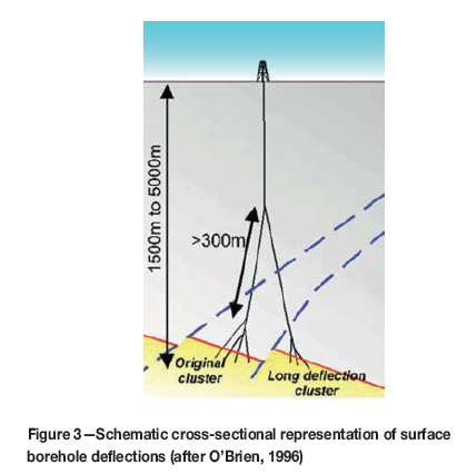
The prohibitive cost involved in deep drilling means that boreholes are normally drilled on a wide spacing, resulting in very low data support. To ensure that as much of this data as possible is available for the estimation process AGA uses 'clusterizing' and 'acceptorizing' processes to try to optimize its availability. The surface boreholes usually consist of multiple reef intersections that are drilled from a single parent diamond borehole. These intersections can range from less than one metre apart up to tens of metres for 'long deflections' (Figure 3).

 

 

Borehole cluster analysis, also known as 'clusterization', aims to determine whether the gold values within the original cluster are sufficiently different from the gold values in the long deflection of the same borehole and as such can be treated independently (O'Brien, 1996; Chamberlain, 1997). The borehole intersection clusters from long deflections are compared to those obtained from original closely spaced intersection values, using the standard statistical analysis of variance approach (O'Brien, 1996). If the analysis of variance shows that the samples from clusters under consideration are not significantly different, then all samples are combined in a 'super cluster' for further use.

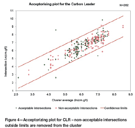
The acceptability of all cored borehole reef intersections is classified according to their mechanical acceptability (completeness of cut, identification of missing chips) and geological acceptability (complete reef, presence of faulting or shearing). The classification of mechanical acceptability is a subjective process and traditionally, if a sample was classified as mechanically unacceptable, the entire intersection would not have been used in estimation. This significantly reduced the number of intersections that could be used and reduced the size of the very limited data-set even further. The 'acceptorizing' process aims to statistically identify which of the unacceptable intersections can be retained and which need to be removed, so as to maximize the number of borehole samples used in the resource estimation process.

The statistical basis of the 'acceptorizing' process is derived from Heyns (1958) and also as expanded and discussed in Dohm (1995), O'Brien (1996), and Chamberlain (1997). Generally there is a mixture of acceptable and non-acceptable intersections within any particular cluster. The logarithms of the ratios of the non-acceptable to acceptable intersection pairs are calculated and 95% confidence limits are set up around the mean of the logarithms. The individual intersections are then plotted against the mean for each cluster (Figure 4). Non-acceptable outliers are then reviewed and removed and the process repeated until the amount of acceptable data that lies outside these confidence limits is at most 5%. Acceptable intersections are not discarded without evidence of significant mechanical loss or geological unacceptability (O'Brien, 1996).

 

 

The CLR borehole data-set consists of 58 clusters after the clusterizing and acceptorizing processes have been carried out.

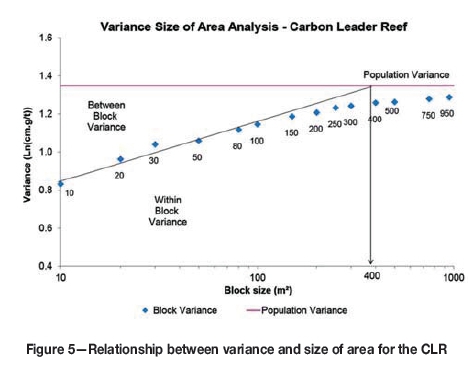
Block size selection and why it is important

The underground chip sampling and surface boreholes are on very different densities, with the chip sampling spacing typically around 5 m x 5 m and the surface boreholes spacing on anything up to 1000 m χ 1000 m. The process of preparing the data for estimation of two different sampling support sizes is a critical aspect of the MCK process. The process taken is to first regularize the chip sampling data into a predetermined block size. The method used to calculate this optimum block size is referred to as the variance size of area analysis (VSOA). The approach ensures that the block size selected is such that the within-block variance is effectively maximized and the between-block variance minimized using the linear extrapolation of dispersion variance. Regularization of chip sampling data on the CLR is performed into 420 m χ 420 m-sized blocks as determined by the VSOA (Figure 5).

 

 

Those 420 m χ 420 m blocks that are not fully informed by the chip sampling, whether due to having too few data points or due to the chip sampling not having a good spatial distribution within the block, are rejected. This data is not, however, lost as it is then created in 'pseudo' boreholes known as clusters. Clusters are created on a 30 m χ 30 m block size for the CLR (approximating a parent borehole and its short deflections) by regularizing the samples within that area. The cluster support data, which now approximates a borehole, is then combined with the real borehole data.

In this way the total data-set is split into block support data and cluster data (inclusive of the boreholes).

Relationship of the mean and variance

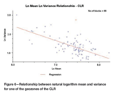
Estimation in MCK is done in natural logarithmic space and therefore the key components to allow the final back-transform are Ln mean and Ln variance. The Ln mean and Ln variance are compared on a scatter plot for the chosen block support data in order to determine whether there is a significant relationship between the two. Ln variance can be estimated from the established relationship using the estimated Ln mean value if a significant relationship is demonstrated. The Ln variance is estimated independently, however, if the relationship is poor.

In some instances a linear relationship, although significant, does not produce reliable results at the final stages of reconciliation and thus it becomes necessary to estimate Ln mean and Ln variance separately (Figure 6). Both Ln mean and Ln variance are estimated for all geozones of the CLR using MCK since the relationship between Ln mean and Ln variance is poor.

 

 

Variography

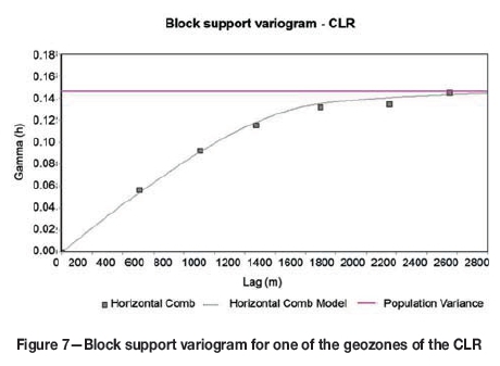
Two sets of variograms are required for estimation, one for block support and one for cluster support. Both sets of variograms are done on Ln mean (value) and Ln variance if the relationship described above is poor.

The block support (420 m χ 420 m) data based on the VSOA process therefore presumes that most or all of the variance is constrained within the block and thus results in a block support variogram model with zero nugget variance. The block support variography is generally characterized by longer ranges, in the order of 1000 m or more (Figure 7), due to the large block sizes.

 

 

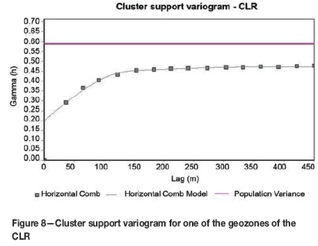
Cluster support variograms (inclusive of the boreholes) are calculated and modelled to determine the nugget variance (Figure 8), with the final cluster variogram used in MCK being a combination of the nugget as modelled from the cluster variogram and the sill and ranges from the block variogram.

 

 

Estimation

MCK of the two support sizes is performed by modification of the kriging matrix to allow different nugget effects; this allows the weighting of the block data differently to the clusters using the combined block and cluster variogram and thus accounting for their support difference (Chamberlain, 1997). The estimation employed for MCK, while termed cokriging, is not strictly cokriging as the data does not need to be collocated nor does it require cross-variograms, with the data for the two support sizes (blocks and clusters) not existing at the same locations. The block size estimated is the same as the block size determined by the VSOA process, in this case 420 m x 420 m.

The number of samples used in MCK has a large influence on the resulting estimate. If the number of samples used is too small (i.e. from a restrictive search neighbourhood), conditional bias could be introduced. Conversely, too many samples could cause undesirable smoothing levels and introduce significant amounts of negative weights, which will also increase the processing time. The amount of samples used in MCK is also controlled by the search neighbourhood. Search parameters used in the MCK process are established through a process of optimization similar to the quantitative kriging neighbourhood analysis (QKNA) process described by Vann et al. (2003). The discretization, numbers of samples, and neighbourhood searches are determined by analysing the kriging variance, regression slope, and percentage of negative weights. This is an iterative process and usually needs to be done for a number of iterations on spatially separated blocks.

The 95% confidence limits are calculated using kriging variance, i.e. Ln 95% lower limit = Ln mean - 1.96 * Ln kriging variance. This methodology is used because the distribution of variances within the 420 m χ 420 m blocks is assumed to approach normality. These values are then input into the CLN model to calculate the limits (Chamberlain, 1997).

Back-transforming the estimates using four-parameter models

Traditional lognormal distributions have been found to be sub-optimal. Sichel (1990) and Sichel et al. (1992) suggested possible alternatives to lognormal distribution models. The suggested four-parameter distributional models were tested against more traditional models by Dohm (1995) and successfully shown to be a more accurate estimation technique than traditional techniques using lognormal theory by Chamberlain (1997).

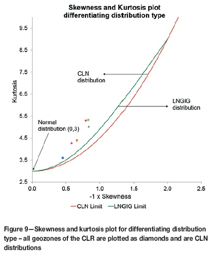
The distribution needs to be defined and fitted once the most appropriate model is determined. Either a four-parameter compound lognormal (CLN) or logarithmic generalized inverse Gaussian distribution (LNGIG) model is used, depending on which distribution model best fits the gold grades and a theoretical test on the shape parameters of the log-transformed values. A theoretical test to differentiate between the two was detailed by Dohm (1995) and can be graphically represented. All the geozones of the CLR follow the CLN distributional model (Figure 9).

 

 

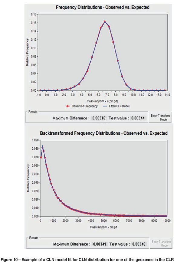
The process of distributional fitting is followed by using classical statistics on the observed data and modelling the distribution using both the histograms of Ln(value) as well as the value (Figure 10). Generally, the fitted CLN model maximum difference (from the observed frequency of the data) needs to be less than the test value for the model fit to be acceptable and so that the Kolmogorov-Smirnov test for goodness of fit does not reject the null hypothesis that the model describes the distribution of the data at the 1% level of significance. The model parameters in the case of the CLN calculated from fitting the distribution used in back-transforming are location (mean), spread (variance), skewness, and kurtosis.

 

 

Estimation is done in natural logarithmic (Ln) space because of the highly skewed gold distribution. The final gold estimates are calculated by back-transforming the estimates using the CLN model in the case of the CLR. The value is estimated by MCK, as is the variance. The skewness and kurtosis parameters are derived from the distribution model of the a priori data as per the Bayesian assumptions.

Regression

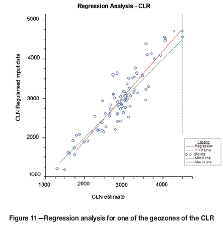
The mean block value of the actual input sampling data at block support is then compared with CLN estimated block values in mined-out areas to determine if a regression effect is present. There is generally a small regression effect still present (Figure 11), thus the back-transformed estimates are regressed using the linear regression observed. Upper and lower limits of the linear regression are identified and the regression is applied to the range of estimates over which the regression is valid. The regression-corrected block estimates are used further in the long-range forecasts of value for the CLR.

 

 

Reconciliations

Numerous methods of reconciliation performed by Chamberlain (1997) validated and demonstrated the effectiveness of MCK. As a final step in the validation process, a similar exercise was followed for the CLR by comparing block estimates over a ten-year period.

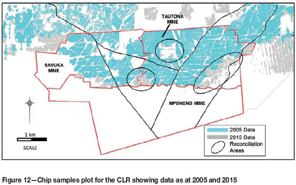
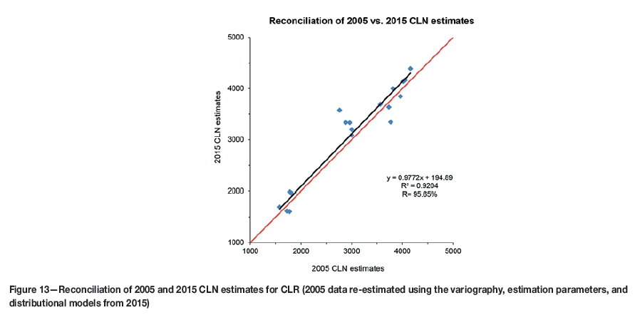
The underground chip sample database from TauTona and neighbouring mines in 2005 consisted of 353 072 points, and 425 917 points in 2015 (Figure 12), reflecting a notable 72 845 increase in samples. The 420 m x 420 m block estimates were compared for the two periods for a selected number of blocks where there had been the largest change in data (Figure 12). There was an initial need to ensure that the estimates used the same geozones, as there has been extensive work on the geological model over time. Thus the 2005 data was re-estimated using the variography, estimation parameters, and distributional models from 2015. This again highlights the importance of accurate and appropriate geological modelling. The 420 m χ 420 m blocks for the two periods are compared in Figure 13. There is a very close correlation between the 2005 and 2015 block estimates for the 18 blocks.

 

 

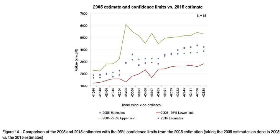
As this reconciliation process provides common critical parameter inputs into the two estimates for 2005 and 2015, it would be a best-case result and could bias the 2005 estimates. Therefore a further reconciliation was done taking the 2005 estimates as done in 2005 vs the 2015 estimates. Figure 14 shows the comparison between the two sets of results, together with the 95% confidence limits from 2005. The MCK estimates from 2015 are well within the 95% confidence limits for the 2005 estimation, indicating that the estimation process used is acceptable and robust for uninformed areas.

 

Conclusion

MCK has a proven and reliable track record and the estimates have been shown to reconcile well over a long timeframe and distance from mining area. Adopting and using a Bayesian approach together with MCK and an appropriate distribution model has resulted in effective and appropriate long-range value forecasts for the CLR. The process is still highly dependent, however, on an accurate geological model as well as a full understanding of the statistical and spatial parameters of the known data. The MCK estimation method has undergone intense scrutiny by a number of external auditors over the past couple of years and proved to be appropriate for the CLR.

 

Acknowledgements

While some of the views expressed in this paper are those of the authors, these opinions have been developed through the wisdom shared by many experienced Mineral Resource professionals over the years. In particular, we are indebted to Christina Dohm, Vaughan Chamberlain, Mike O'Brien, Patrick Rice, and Robert Lavery on their work leading to the established practice of MCK and training therein.

 

References

AngloGold Ashanti. 2014. Mineral Resource and Ore Reserve Report. 192 pp.         [ Links ]

Chamberlain, V.A. and O'Brien, M.F. 1995. Strategic ore evaluation: current techniques used by the Anglo American Corporation. Presented at a meeting of the South African Institute of Mining and Metallurgy, Johannesburg.         [ Links ]

Chamberlain, V.A. 1997. The application of macro co-kriging and compound lognormal theory to long range grade forecasting for the Carbon Leader Reef. MSc (Eng) thesis, University of the Witwatersrand, Johannesburg.         [ Links ]

Dohm, C.E. 1995. Improvement of ore evaluation through identification of homogenous areas using geological, statistical and geostatistical analyses. PhD thesis, Faculty of Engineering, University of the Witwatersrand, Johannesburg.         [ Links ]

Heyns, A.J.A. 1958. A problem in borehole valuation. Unpublished paper read at the South African Statistical Association.         [ Links ]

Krige, D.G., Kleingeld, W.J., and Oosterveld, M.M. 1990. A priori parameter distribution patterns for gold in the Witwatersrand Basin to be applied in borehole valuation of potential new mines using Bayesian geostatisical techniques. Proceedings of the 22nd International Symposium on the Application of Computers and Operations Research in the Mineral Industry (APCOM), Berlin, 17-21 September 1990. Technische Universitát Berlin. pp. 715-726.         [ Links ]

O'Brien, M.F. 1996. Making maximum use of limited sampling data from deep boreholes: verification techniques. Geostatistics Wollongong '96 - Proceedings of the 5th International Geostatistical Congress. Baafi, E.Y. and Schofield, N.A. (eds.). Kluwer Academic Publishers. pp. 792-798.         [ Links ]

Sichel, H.S. 1949. Mine valuation and maximum likelihood, MSc thesis, University of the Witwatersrand, Johannesburg.         [ Links ]

Sichel, H.S. 1990. The log generalised inverse gaussian distribution and the compound lognormal distribution, Unpublished course notes, Ore Evaluation Department, Anglo American Corporation of South Africa.         [ Links ]

Sichel, H.S., Kleingeld, W.J., and Assibey-Bonsu, W. 1992. A comparative study of three frequency-distribution models for use in ore evaluation. Journal of the South African Institute of Mining and Metallurgy, vol. 92, no. 4. pp. 91-99.         [ Links ]

Vann, J., Jackson, S., and Bertoli, O. 2003. Quantitative kriging neighbourhood analysis for the mining geologist - a description of the method with worked case examples. Proceedings of the Fifth International Mining Geology Conference, Bend igo, Victoria, 17-19 November 2003. Australasian Institute of Mining and Metallurgy, Melbourne. pp. 215-223.         [ Links ]

Vann, J. 2009. Quantitative Group Mineral Resource review of the Carbon Leader Reef, West Wits, South Africa. AngloGold Ashanti. Unpublished document.         [ Links ]

 

 

This paper was first presented at, The Danie Krige Geostatistical Conference 2015, 19-20 August 2015, Crown Plaza, Rosebank.