PAPERS - SLOPE STABILITY CONFERENCE

 

Designing for extreme events in open pit slope stabilty

 

 

L. Lorig

Itasca

 

 

---

SYNOPSIS

Two types of extreme event, earthquakes and rainfall, potentially affect open pit slope stability. In the case of earthquakes, there are rather well-developed analysis procedures and acceptability criteria. The analysis procedures relate mainly to selection of the dynamic loading either through design earthquakes and/or pseudo-static seismic coefficients. The acceptance criteria are typically expressed in terms of a minimum safety factor in pseudo-static analyses. The acceptance criteria are often promulgated by governments despite the fact that no open pit slope has ever been adversely affected by an earthquake. This paper explains why open pit slopes are seemingly more resistant to dynamic loads than natural landforms, which can experience catastrophic landslides.
Extreme rainfall events are much more likely to cause open pit slope problems than earthquakes. Two types of problem are common - slope erosion and slope instability. Slope erosion is often mitigated by appropriate surface water controls. Slope instability due to elevated transient water pressures is more difficult to mitigate. Analysis procedures and acceptability criteria are rare. This paper will discuss the mechanisms for rainfall-induced slope instability, as well as analysis methods. Examples will be discussed and analysis methods are proposed.

Keywords: slope stabililty, analysis methods, acceptability criteria, extreme rainfall

---

 

 

Introduction

Two types of extreme event, earthquakes and rainfall, potentially affect open pit slope stability. In the case of earthquakes, there are rather well-developed analysis procedures and acceptability criteria. The analysis procedures relate mainly to selection of the dynamic loading either through design earthquakes and/or pseudo-static seismic coefficients. The acceptance criteria are typically expressed in terms of a minimum safety factor in pseudo-static analyses. The acceptance criteria are often promulgated by governments (e.g., Peru, Chile) despite the fact that no open pit slope has ever been adversely affected by an earthquake. This paper explains why open pit slopes are seemingly more resistant to dynamic loads than natural landforms, which can experience catastrophic landslides.

Extreme rainfall events are much more likely to cause open pit slope problems when compared to earthquakes. Two types of problems are common - slope erosion and slope instability. Slope erosion is often mitigated by appropriate surface water controls. Slope instability due to elevated transient water pressures is more difficult to mitigate. Analysis procedures and acceptability criteria are rare, but do exist. In Peru, for example, slopes are required by law to be designed for a 100-year storm.

Thus it seems that there is disproportional design attention given to these two extreme events. Large slope displacements and even failure are often preceded by periods of heavy rainfall, yet little, if any design attention is paid to rainfall (or in some cases snowmelt). If nothing else, this paper aims to raise awareness of the need to consider the impact of the amount and rate of rainfall in the design process.

 

Earthquakes and open pits

Failure of rock slopes is a complex phenomenon, often involving failure of rock bridges and sliding on pre-existing joints. Stress changes are induced in slopes by earthquake movements. Combined with existing static stresses, these additional dynamic stresses may exceed the available strength along a potential sliding surface (formed of the rock bridges and pre-existing joints) and cause failure. These failures can either be in the form of slides and rockfalls, where the material is broken into a large number of small pieces, or coherent slides, where a few large blocks translate or rotate on deep-seated failure surfaces. Glass (2000) notes that while shallow slides and rockfalls are quite common during earthquakes (Harp and Jibson, 1995, 1996), the correlation of seismic shaking with open pit slope failures is much less compelling, and he is not aware of any large, deep, coherent open pit slope failures that have been attributed to earthquake-induced shaking. Although earthquakes apparently pose a low-probability risk to open pit mines, given their relatively shorter design lifetime in comparison to natural slopes, and small landslides and rockfalls cause little disruption to mining operations, a deep coherent failure could still have a profound effect.

Because mining regulations often require investigation of slope stability in response to earthquake loading, relatively simple quasi-static analyses are typically carried out for open pit mines. It is widely recognized (e.g. Kramer, 1996) that the quasi-static analysis of the effect of seismic shaking on stability of slopes is inadequate and incorrect (and usually too conservative). Thus, open pit mine designers often defer to empirical evidence when considering seismic hazard in open pit slope design.

It is important to understand and explain the relatively good performance of open pit slopes as opposed to extensive evidence of landslides during historical earthquakes, but also to determine the conditions when open pit slope stability can be at risk during the seismic shaking. Damjanac et al. (2013) provide, based on a mechanistic approach (using numerical models), a rationale for why field observations indicate relatively small effects of earthquakes on the stability of open pit slopes, and also investigate the level of conservatism in the predictions of the quasi-static analyses as a function of important ground motion parameters.

Large open pits versus natural slopes

The main differences between large open pit slopes and natural slopes that are believed to be reasons for better performance of large open pit slopes during earthquakes are summarized below (after Damjanac et al., (2013).

a. Infrequent occurrence of strong earthquakes during the mine's lifetime. The life of a mine is relatively short compared to the recurrence periods of large earthquakes (M_w>6.5). Natural slopes are hit by numerous strong earthquakes, resulting in damage accumulation and gradual reduction in the safety margin

b. Natural slopes exist at a wide range of conditions and wide range of factors of safety (FoS), with some of them being metastable (close to FoS = 1.0) under static conditions. Typically, open pits are designed to have a static FoS of around 1.2 or greater. As a result, some natural slopes are likely to fail when subject to additional dynamic loading from earthquakes

c. Earthquakes cause failure of some of the natural slopes that are close to static equilibrium. However, most natural slopes do not fail. In fact, a small fraction of all natural slopes fail during even very strong earthquakes.

d. Open pits are typically excavated in relatively strong, competent rocks. Natural slopes are comprised of rock and soil with different states of degradation and weathering and are susceptible to softening mechanisms.

e. As explained later, topographic amplification is greater in natural slopes than in open pits

f. Also, as explained later, wave amplification due to heterogeneities is much greater in natural slopes than open pits.

For the reasons described above, natural slopes are at a disadvantage when subjected to seismic loading, both in terms of higher additional demand induced by dynamic stresses and lower extra capacity available in material strength to meet that demand. In the following sections, these factors are quantified. For the same magnitude earthquake, the actual shaking and dynamic stresses induced in the slope are functions of slope geometry (surface topography) and geological profile (variation of mechanical properties with depth). Both these effects are studied using two- and three-dimensional numerical models as described below.

Induced dynamic stresses caused by seismic shaking

One aspect of the problems caused by earthquakes is the increased demand due to induced dynamic stresses caused by seismic shaking. This can be due to either geometric effects (topographic amplification) or material heterogeneity (e.g., softer material underlain by hard rock). Both of these effects are evaluated in this section by means of continuum elastic numerical simulations. Damjanac et al. (2013) investigated conditions when dominant wavelengths and the characteristic height of the pit are large relative to any structure in the rock mass, which can be approximated as a continuum. The finite-difference software packages FLAC (Itasca, 2011) and FLAC3D (Itasca, 2012) were used in the study.

Topographic amplification

It has been observed in many earthquakes that the formation geometry plays a critical role in site response and may lead to trapping of seismic energy in a certain region or channelling it away. This can lead to amplification of ground motion in some areas while moderating it in others (Raptakis et al., 2000; Bouckovalas and Kouretzis, 2001; Assimaki and Kausel, 2007). The effect of topography on wave amplification is investigated for both two- and three-dimensional geometries as explained in Appendix A.

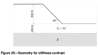
Stiffness contrast

Another reason for amplification of seismic waves is the presence of heterogeneities (e.g., typically softer materials on top of more competent rock). Seismic waves propagating downward after reflection at the free surface are trapped between the free surface and more competent rock, leading to a very high amplification ratio. In Appendix B, the effect of both horizontal layering and vertical heterogeneities (e.g., orebody) is examined.

Dynamic safety factor

The reduction in FoS due to additional demand induced by seismic shaking is quantified and correlated with different earthquake intensity parameters. A suite of real ground motions was selected with a wide range of peak ground accelerations (PGAs), peak ground velocities (PGVs), durations of shaking, and frequency content. The model geometry is the same as for 2D elastic simulations (Appendix A) with a slope height of 500 m. The analysis is carried out for two different overall slope angles: 45° and 35°. The rock is modelled as a dry elasto-plastic material using a Mohr-Coulomb yield criterion with strength values corresponding to typical values for fractured rock. For the 45° slope, a cohesion of 0.5 MPa and a friction angle of 45° is used. For the 35° slope, a cohesion of 0.37 MPa and a friction angle of 37° is used. A Poisson's ratio of 0.2 is used for both cases. The lateral stress is initialized using a lateral stress coefficient of =0.25. These parameters result in a static factor of safety (FoS_s) of 1.5 for both slopes.

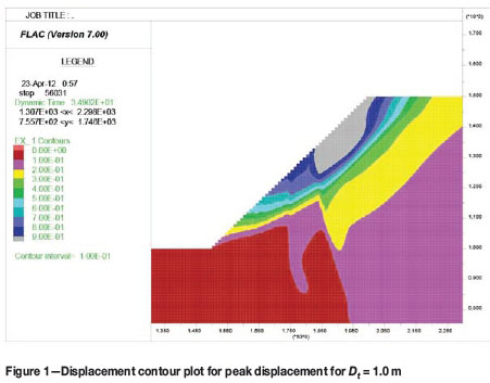
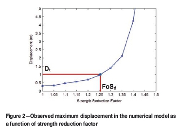
To calculate the dynamic factor of safety (FoS_d), a threshold displacement (D_t) above which the slope is considered to have failed is chosen. This chosen displacement corresponds to shear strains that are expected to cause significant loss in rock mass strength. Two values are considered: D_t= 0.5 m and D_t=1.0 m. A dynamic analysis is performed using each ground motion (both horizontal and vertical components) and the maximum displacement on slope is monitored. If the displacement is less than the threshold, strength properties (cohesion and friction angle) are reduced in increments and the analysis is rerun until the permanent earthquake-induced displacements are greater than the threshold. This strength reduction factor is denoted as the FoS_d for that ground motion. A typical displacement contour plot for maximum displacement D_t= 1.0 m is shown in Figure 1. A typical plot of maximum displacement as a function of strength reduction factor highlighting the calculation of FoS_d is shown in Figure 2.

 

 

 

 

The FoS_d is then normalized by the FoS_s, and the ratio is correlated with different earthquake intensity parameters.

The following earthquake intensity parameters are correlated with the dynamic factor of safety.

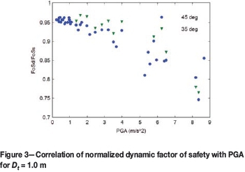
1. Peak ground acceleration (PGA): maximum value of absolute acceleration. The correlation is shown in Figure 3 for Dt = 1.0 m

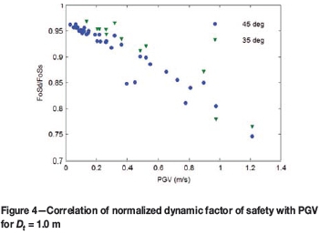
2. Peak ground velocity (PGV): maximum value of absolute velocity. The correlation is shown in Figure 4 for Dt = 1.0 m

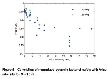
3. Arias intensity (I_a): time integral of square of ground acceleration (in m/s²):

 

 

 

 

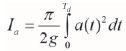
where g is the acceleration due to gravity and a(t) is the acceleration at time instant t.

The correlation is shown in Figure 5 for D_t= 1.0 m.

 

 

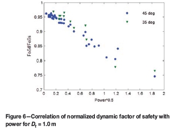
4. Power: time integral of square of ground velocity:

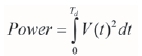
where V(t) is the velocity at time instant t.

The correlation is shown in Figure 6 for D_t= 1.0 m.

 

 

5. Cumulative absolute velocity (CAV): time integral of absolute value of acceleration

The correlation is shown in Figure 7 for D_t= 1.0 m.

 

 

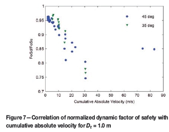
The correlation of normalized dynamic factor of safety with both Arias intensity and cumulative absolute velocity (CAV) is poor. Some correlation is obtained with peak ground acceleration (PGA), but the scatter increases significantly for higher levels of PGA. The best correlation is obtained with PGV and power, with PGV performing slightly better. Good correlation is obtained for both levels of threshold displacement (0.5 m and 1 m) when PGV is used. Thus, PGV is found to be a better indicator of seismic damage to slopes than PGA, which is used in conventional methods.

Conventional pseudo-static approach

The results from numerical analysis are compared with the pseudo-static approach commonly employed for determining the dynamic factor of safety for slopes. The pseudo-static method involves running a static analysis with a horizontal component of acceleration a_h, = k_sg where k_sis the seismic coefficient and is correlated with earthquake magnitude (Pyke, 2001) and peak ground acceleration. To compare the results directly, pseudo-static analyses were carried out and the factor of safety was calculated for different seismic coefficients. The results are shown in Figure 8.

 

 

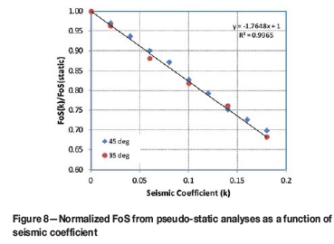
For every earthquake motion used in numerical analysis in the previous section, a dynamic factor of safety was determined. Using the chart in Figure 8, a seismic coefficient that would give the same factor of safety in pseudo-static analysis for that earthquake was determined. These seismic coefficients are normalized by PGA and plotted against the earthquake magnitude. The cases with very low PGA are excluded as they are prone to large errors when normalized. The results are compared with recommendations by Pyke (2001) as shown in Figure 9.

 

 

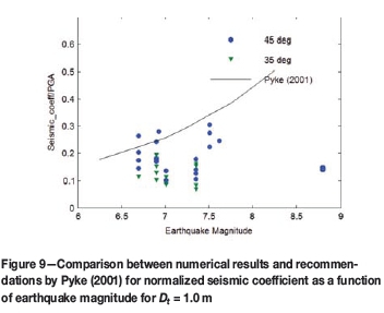
The results indicate that there is no significant correlation between the seismic coefficient and earthquake magnitude. However, for the most part, the recommendation by Pyke (2001) corresponds to the upper bound and is conservative. While this approach may work fine for low-magnitude earthquakes, it can lead to an over-conservative design for larger-magnitude earthquakes. As discussed in the next section, using another ground motion parameter such as PGV instead of magnitude may help in better estimation of the dynamic factor of safety for such cases. It is logical that PGV might be better because velocity relates directly to stress.

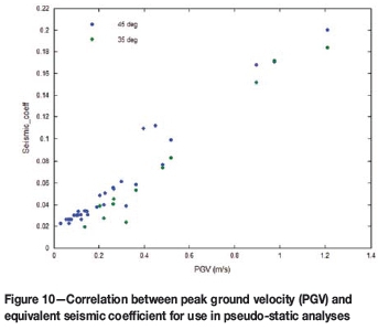
Improved pseudo-static approach

As discussed above, Damjanac et al. (2013) reported results for a two-dimensional fully dynamic study involving homogeneous slopes 500 m high at 35° and 45° slope angles for 20 recorded ground motions (for earthquakes covering ranges of magnitudes, durations, and epicentre distances). The study showed that reduction in the dynamic factor of safety (FoS_d) does not correlate well with the PGA and event magnitude. Consequently, the charts and empirical formulae for calculation of pseudo-static seismic coefficient currently used in industry for pit design and assessment of the seismic hazard are inadequate. The study also showed that currently used seismic coefficients typically overestimate the seismic hazard for the pit slopes. However, in a few cases, that hazard is underestimated. Full dynamic analyses indicate that reduction in the FoS due to dynamic loading best correlates with PGV, which is one of the earthquake intensity measures. The pseudo-static seismic coefficients that result in the same FoS as calculated from full dynamic analysis for the considered ground motions are shown in Figure 10. as functions of PGV. Clearly, the correlation is very good. More research is needed to generalize the process into a more accurate and rigorous, but simple, methodology for calculating seismic coefficient to be used in the pit design and assessment of the earthquake hazard.

 

 

Extreme rainfall and open pits

Extreme rainfall events are among the most common causes of slope instability in open pits. As discussed in this section, extreme rainfall can adversely affect both soil and rock slopes, although the mechanisms are different.

Soil slopes

Soil slopes are affected by extreme rainfall in one of two ways - erosion and/or loss of apparent cohesion (suction).

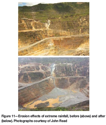
Erosion

Soil erosion due to rainfall is probably the most common consequence of an extreme rainfall event. An example of soil erosion is shown in Figure 11. Erosion is probably best handled by providing an effective surface water management system.

 

 

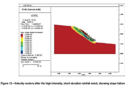
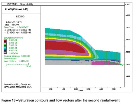
Stability in unsaturated conditions

The presence of capillary pressure in unsaturated soils can have a major impact on the stability of a slope. Capillary forces hold fine particles together and can impart additional cohesion to the soil. The apparent cohesion provided by the capillary forces usually decreases as the soil saturation increases. With saprolites and other granular soils, strong negative pore pressures (soil suction) are developed when the moisture content is below about 85%. This behaviour explains why many saprolite slopes remain stable at slope angles and heights greater than would be expected from typical effective stress analysis. It also explains why these slopes may fail after prolonged rainfall even without the development of excess pore pressures or reaching 100% saturation (Fourie and Haines, 2007). While a rainfall event of low intensity and long duration may under certain conditions be beneficial to the stability of the slope, a high-intensity, short-duration event may promote a buildup of saturation and induce slope failure. Detournay and Hart (2008) provide the theoretical background and use numerical simulations with FLAC (Itasca, 2011) to illustrate the relationship between rate of infiltration from precipitation and stability in a silty slope. They used a simplified framework, based on Mohr-Coulomb model for the soil, generalized Bishop effective stress (Nuth and Laloui, 2007; Wang et al., 2015), and van Genuchten laws relating capillary pressure and permeability to saturation (van Genuchten, 1980) to show the impact of intensity and duration of a rainfall event on the stability of a slope. Generic geometry and material properties were used for the slope. It was shown that a rainfall event of low intensity and long duration was not detrimental to slope stability, provided that the additional cohesion imparted to the soil by the capillary forces was sufficient. On the other hand, a rainfall event of high intensity and short duration was responsible for slope failure (see Figure 12). In this case, the behaviour was explained by an increase in soil saturation (see Figure 13) accompanied by a decrease in the capillary forces, intensity, causing an apparent decrease in soil cohesion. A similar discussion and example is provided by Garcia et al. (2011).

 

 

 

 

Predicting rainfall-induced slope instability using simplified methods

Numerical analyses, such as shown in the previous section, are complex due to the nonlinearity of the hydraulic and soil constitutive behaviour at play. In addition, the actual geometry of the slope may add another level of complexity. A simplified approach to handle the problem is desirable, if practical guidance is to be the outcome of the analysis.

One possibility is to simplify the geometry of the problem, without compromise to the established hydraulic and soil behaviour. For example, the case of an infinite slope has been adopted by several authors, including Fourie (1996), Iverson (2000), Collins (2004), and Tsai et al. (2008), to name a few.

Fourie (1996) provides a methodology based on statistical rainfall records together with a simplified method to simulate the rate of infiltration. The methodology includes rainfall intensity, duration, and antecedent conditions in assessing slope stability based on Pradel and Raad's (1993) approximate method. The process starts with the rainfall data expressed in terms of rainfall intensity, duration, and return period (Figure 14).

 

 

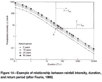
The next step is to determine the minimum rainfall intensity (I_min) that exceeds the infiltration rate of the soil and must last long enough (T_min) to saturate the soil to a depth z_wmeasured perpendicular to the slope.

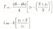
where θ_s and θ_o are the saturated and in situ volumetric water content respectively, k is the coefficient of hydraulic conductivity of the soil in the wetted zone and S is the wetting-front capillary suction (metres of water).

The relations are shown for a hypothetical example in Figure 14 where all rainfall events with an intensity and duration that plot within the box in the top right-hand corner will be sufficient to saturate soil to a depth z_w. The final step is to compute the safety factor of the slope for the saturated soil depth, z_w. Within the saturated depth, the matric suction (capillary pressure) should be reduced to a minimum value.

Rock slopes

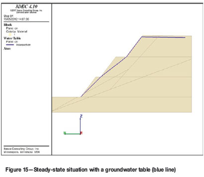
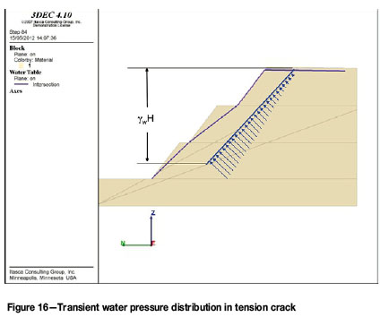
The behaviour of rock slopes is significantly different from that of soil slopes during extreme rainfall events. Whereas soil slopes may fail due to loss of apparent cohesion, rock slopes generally fail due to high transient water pressures in open fractures, particularly tension-induced fractures (tension cracks) as described below. Transient pressures equivalent to 40 m of water have been measured at some mines.

Transient water pressure in tension cracks

Consider, for example, the steady-state condition shown in Figure 15. Under steady-state conditions, the pressure at any point along a structure is approximated by the product of the vertical depth below the groundwater table and the unit weight of water. Under transient conditions, a tension crack may quickly fill with water, producing the condition shown in Figure 16. The water pressure in the tension crack in Figure 16 is significantly higher than in Figure 15. In this particular case, the slope in Figure 15 had a safety factor of 1.18, whereas the slope in Figure 16 had a safety factor of 1.01.

 

 

 

 

Seasonal infiltration effects

In most cases when we consider extreme rainfall events, we think about durations of days or weeks. However, extreme rainfall events can also be seasonal, with rainfall occurring over months. This section discusses the effect of seasonal rainfall on a slope simulated as an equivalent continuum.

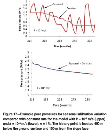
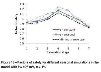
The effect of seasonal infiltration in a rock slope was examined by Hazzard et al. (2011) by alternating the rate of infiltration between zero for six months, and twice the average infiltration rate for six months. Example pore pressure histories are shown in Figure 17 for models with k = 10^-6 m/s and k = 10^-8 m/s. It is clear that the high-permeability model is affected greatly by the seasonal variations, whereas the low-permeability model is not. To examine the effect of the seasons on FoS, four different scenarios were simulated to consider different offsets for the start of the wet season. The FoS for the different seasonal simulations in one model are shown in Figure 18. Factors of safety were calculated nine months after each excavation. Depending on the start of the wet season, this may or may not correspond to peak transient pore pressures. However, it is possible to construct an envelope encompassing the minimum FoS for the four different scenarios; then it is possible to pick the peak pressure state for each excavation stage. Next, it is possible to calculate the average FoS over stages 1 to 6 for this minimum envelope and compare the results to the FoS calculated for a constant infiltration rate. Such an analysis clearly shows that the seasonal variations essentially have no effect on the FoS for low permeabilities and/or high excavation rates. However, for high permeabilities and/or low excavation rates, the seasonality may result in a decrease in FoS of up to 8%. Similar results are obtained for the other infiltration rates, except that as q decreases, the effect of seasonality becomes even less severe. For q = 0.3 m/a, the maximum decrease in FoS caused by seasonality is only about 2.5% compared to constant q.

 

 

 

 

Concluding remarks

When it comes to earthquakes, it appears that stability analyses are largely unnecessary unless required by law. Possible exceptions might include mined slopes on the sides of steep, elevated topography where amplification affects may be important. If dynamic analyses are performed, time-domain numerical analyses are preferred over pseudo-static analyses due to their inherent ability to reproduce transient seismic forces. If pseudo-static analyses are performed, consider selecting seismic coefficients using peak particle velocity (PPV) rather than peak ground acceleration (PGA).

Designing for extreme rainfall events starts with designing stable slopes for 'normal' conditions such that tension cracks are minimized to the extent practicable and thus limiting the opportunities for water to enter cracks. The next step is to provide good surface drainage so that water does not erode and/or infiltrate slopes. Even with these mitigation measures, there is a need to consider the possibility that extreme rainfall may adversely affect slopes. Selection of appropriate acceptability criteria for extreme rainfall depends on risk tolerance, but it seems that a safety factor of at least unity under extreme rainfall conditions (e.g., 24-hour duration and 100-year return period) is a reasonable starting point. Stability of soil slopes can by evaluated using an approximate method described in the paper or numerical models. For hard rock slopes, the rainfall-induced transient pressures should be considered either in an equivalent continuum rock mass and/or in explicit discontinuities.

 

Acknowledgements

The author would like to acknowledge Itasca colleagues Branko Damjanac, Christine Detournay, Roger Hart, Varun, Pedro Velasco and others for their important contributions to this paper. The author would also like to thank the Large Open Pit Consortium and Commonwealth Scientific Industrial and Research Organization (CSIRO) for the financial support provided for the study of earthquake effects on large open pits. Finally, the author would like to thank professional colleagues, including Alan Guest, John Read, Peter Stacey, and Christian Holland, Geoff Beale and others, that provided valuable insights.

 

References

Assimaki, D. and Kausel, E. 2007. Modified topographic amplification factors for a single-faced slope due to kinematic soil-structure interaction. Journal of Geotechnical and Geoenvironmental Engineering, vol. 133, no. 11. pp.1414-1431.         [ Links ]

Bouckovalas, G.D. and Kouretzis, G. 2001. Review of soil and topography effects in the September 7, 1999 Athens (Greece) earthquake. Proceedings of the Fourth International Conference on Recent Advances in Geotechnical Earthquake Engineering and Soil Dynamics and Symposium in Honor of Professor W. D. Liam Finn, San Diego, California, 26-31 March.         [ Links ]

Collins, B. and Znidarcic, D. 2004. Stability analyses of rainfall induced landslides. Journal of Geotechnical and Geoenvironmental Engineering, vol. 130, no. 4. pp. 362-372. DOI: 10.1061/(ASCE)1090-0241(2004)130:4(362)        [ Links ]

Damjanac, B., Varun, and L. Lorig. 2013. Seismic stability of large open pit slopes and pseudo-static analysis. Proceedings of the International Symposium on Slope Stability in Open Pit Mining and Civil Engineering (Slope Stability 2013), Brisbane, Australia, September, 2013. Dight, P. (ed.). Australian Centre for Geomechanics, Perth, Australia. pp. 1203-1216,         [ Links ]

Detournay, C. and Cundall, P. 2001. Numerical modeling of unsaturated flow in porous media using FLAC. FLAC and Numerical Modeling in Geomechanics. Proceedings of the 2nd International FLAC Symposium, Lyon, France, 29-31 October 2001. Billaux, D., Detournay, C., Hart, R., and Rachez, X. (eds.). A.A. Balkema, Lisse.         [ Links ]

Detournay, C. and Hart, R. 2008. Stability of a slope in unsaturated conditions. Continuum and Distinct Element Numerical Modeling in Geo-Engineering. Proceedings of the 1st International FLAC / DEM Symposium, Minneapolis, August 2008. Sainsbury, D., Hart, R., Detournay, C., and Nelson, M. (eds.). Paper no. 03-03. Itasca Consulting Group, Minneapolis.         [ Links ]

Fourie, A.B. 1996. Predicting rainfall-induced slope instability. Geotechnical Engineering, vol. 119, no. 4. pp. 211-218.         [ Links ]

Fourie, A.B. and Haines, A. 2007. Obtaining appropriate design parameters for slopes in weathered saprolites. Slope Stability 2007. Proceedings of 2007 International Symposium on Rock Slope Stability in Open Pit Mining and Civil Engineering. Potvin, Y. (ed.). Australian Centre for Geomechanics, Perth. pp. 105-116.         [ Links ]

Garcia, E.F., Riveros, C.A., and Builes, M. A. 2011. Influence of rainfall intensity on infiltration and deformation of unsaturated soil slopes. Dyna, no. 170. pp. 116-124.         [ Links ]

Glass, C.E. 2000. The influence of seismic events on slope stability. Slope Stability in Surface Mining. Society for Mining, Metallurgy and Exploration, Littleton, CO. pp. 97-105.         [ Links ]

Harp, E.L. and Jibson, R.W. 1995. Inventory of landslides triggered by the 1994 Northridge, California earthquake. US Geological Survey open file Report 95-213. 17 pp.         [ Links ]

Harp, E.L. and Jibson, R.W. 1996. Landslides triggered by the 1994 Northridge, California earthquake. Bulletin of the Seismological Society of America, vol. 86, no. 1B. pp. S319-S332.         [ Links ]

Hazzard, J., Damjanac, B., Lorig, L., and Detournay, C. 2011. Guidelines for groundwater modelling in large open pit mine design. Slope Stability 2011: Proceedings of the International Symposium on Rock Slopes in Open Pit Mining and Civil Engineering, Vancouver, September 2011. Eberhardt, E. and Stead, D. (eds.). Canada Rock Mechanics Association, Vancouver. Paper no. 114.         [ Links ]

Itasca Consulting Group, Inc. 2011. FLAC: Fast Lagrangian Analysis of Continua, version 7.0. User's manual.         [ Links ]

Itasca Consulting Group, Inc. 2012. FLAC3D: Fast Lagrangian Analysis of Continua in 3D, version 5.0. user's manual.         [ Links ]

Iverson, R.M. 2000. Landslide triggering by rain infiltration. Water Resources Research, vol. 36, no. 7. pp. 1897-1910.         [ Links ]

Kramer, S. L. 1996. Geotechnical Earthquake Engineering. Prentice-Hall.         [ Links ]

Nuth, M. and Laloui, L. 2007. Effective stress concept in unsaturated soils: clarification and validation of a unified framework. International Journal for Numerical and Analytical Methods in Geomechanics, vol. 32. pp. 771--801.         [ Links ]

Pradel, D. and Raad, G. 1993. Effect of permeability on surficial stability of homogeneous slopes. Journal of Geotechnical Engineering, vol. 119, no. 2. pp. 315-332.         [ Links ]

Pyke, R. 2001. Selection of seismic coefficients for use in pseudo-static analyses. TAGAsoft Limited. www.tagasoft.com/discussion/article2.html        [ Links ]

Raptakis, D., Chavez-Garcia, F.J., Makra, K., and Pitilakis, K. 2000. Site effects at Euroseistest-I. Determination of the valley structure and confrontation of observations with 1D analysis. Soil Dynamics and Earthquake Engineering, vol. 19. pp. 1-22.         [ Links ]

Tsai, T-L., Chen, H-E., and Yang, J-C. 2008. Numerical modeling of rainstorm-induced shallow landslides in saturated and unsaturated soils. Environmental Geology, vol. 55. pp. 1269-1277.         [ Links ]

Van Genuchten, M.TH. 1980. A closed form equation for predicting the hydraulic conductivity of unsaturated soils. Soil Science Society of America Journal, vol. 44. pp. 892-898.         [ Links ]

Wang, L, Liu, S., Fu, Z., and Li, Z. 2015. Coupled hydro-mechanical analysis of slope under rainfall using modified elasto-plastic model for unsaturated soils. Journal of Central South University, vol. 22. pp. 1892-1900.         [ Links ]

 

 

© The Southern African Institute of Mining and Metallurgy, 2016. ISSN 2225-6253.
This paper was first presented at the, International Symposium on Slope Stability in Open Pit Mining and Civil Engineering 2015, 12-14 October 2015, Cape Town Convention Centre, Cape Town.

 

 

Appendix A - Effect of topography on dynamic wave amplification (from Damjanac et al., 2013)

A.1 Two-dimensional effects

Based on typical configurations of open pit mines and natural slopes, three simplified slope geometries, shown in Figure 19, are studied using two-dimensional (2D) numerical analyses. These are (a) a single slope model that is representative of a natural slope or a wide pit, (b) a pit model representative of open pits, and (c) a hill model representative of most natural slopes. These models can be expressed in terms of following parameters:

 

 

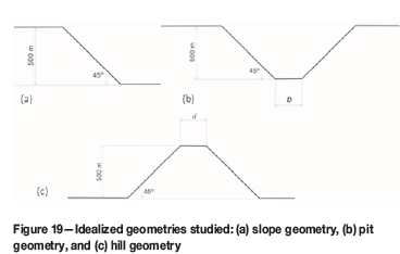
1. Height of slope (H), assumed to be 500 m for the simplified geometry

2. Angle of slope (θ), assumed to be 45 degrees for the simplified geometry

3. Width of basin (b) or ridge crest (d), varied from 0.0 to 2.0 times the slope height.

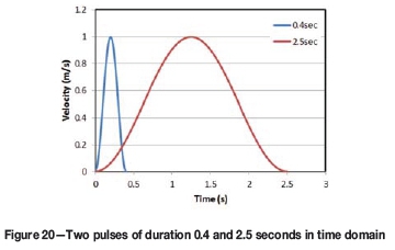
To simulate seismic excitation, single pulses are used as input motion. The pulses are characterized by their duration T as

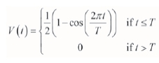
where V(t) is the particle velocity at time t.

The signal contains frequencies in the range 0 to 2/T Hz. Figure 20 shows the time history for two pulses with T = 0.4 seconds and 2.5 seconds. The motion is applied at the base of the model as a shear stress time history to simulate an incoming wave. Quiet boundaries are used at the base to avoid any reflection of outgoing waves back into the model. Appropriate forces obtained from one-dimensional site response are applied at the lateral boundaries to simulate free-field behaviour correctly. A density of 2500 kg/m³ and shear wave velocity of 1000 m/s are assumed for the rock.

 

 

The simulations are carried out for pulse durations ranging from 0.1 to 10 seconds. The results are compared in terms of peak velocity obtained at the surface. Two parameters are recorded for each simulation, the first being the peak velocity on the slope surface, and the second being the peak velocity at the ground surface throughout the model. For short duration pulses, both parameters are the same as maximum velocity is obtained on the slope surface itself. However, for longer duration pulses, the maximum velocity is obtained behind the crest of the slope as shown in Figure 21.

The results for slope and pit geometries were found to be almost identical, irrespective of the width parameter (b). This is due to the fact that incident waves travel up the slope and, given the shape of pit geometry, are reflected away from the pit. As a result, there is no interaction between the waves incident on two sides of the pit. Therefore, when comparing results, only the slope geometry results are shown and are taken to be representative of pit geometry as well.

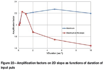
The results are presented as the amplification factor (i.e., the ratio of PGV observed to the PGV for the incoming motion). The results are plotted as a function of the inverse of pulse duration, which is indicative of the frequency content of the ground motion. The frequency can also be normalized and written in dimensionless form as H/V_sT, where V_sis the shear wave velocity of rock at surface and H is the slope height.

The results for the slope/pit geometry are shown in Figure 22. As can be seen from the results, for long duration pulses (i.e., pulses containing lower frequencies), peak velocity is observed on the slope surface itself. For the limiting case of an infinitely long pulse, the amplification is 2.0, which is the same as the free surface amplification (i.e., the topographic effects are negligible). As the frequency increases, the peak surface velocity also increases with the peak being observed at a frequency of 0.8 Hz (H/V_sT = 0.4). A further increase in frequency does not lead to any significant increase in peak ground velocity. Instead, the location of the peak velocity moves away from the slope surface to behind the crest of the slope. The maximum amplification observed for the pit geometry is around 2.24, which is not a significant increase compared to the free surface amplification factor of 2.0.

 

 

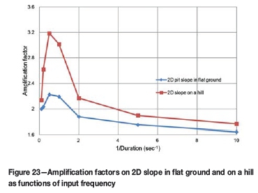
For the hill geometry, the results are a function of the width 'd'. As width increases, →∞, the amplification decreases and the amplification curve approaches the slope geometry case. Maximum amplification is observed for the case where d = 0. A comparison between amplification curves for peak velocity on the slope surface for the hill geometry (with d = 0) and slope geometry are shown in 23. The amplification curve for the hill geometry shows a similar shape as for the slope geometry with peak amplification occurring at 0.8 Hz, which corresponds to a dimensionless frequency of 0.4. However, the amplification ratio is much higher with peak amplification of 3.2. This is due to the 'focusing effect' of the hill geometry where the waves incident on the slope are directed toward the crest from both sides and result in energy from a wide base at the bottom being focused in a small area at the top. Thus, natural slopes experience much higher velocities (and acceleration) due to topographic amplification.

A.2 Three-dimensional effects

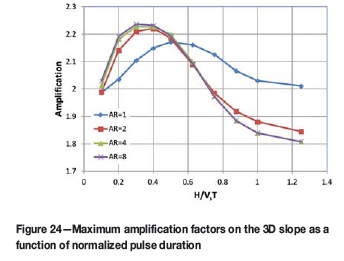
The next step was to evaluate the effect of three-dimensional pit shapes on the amplification ratio. The pit is modelled as an ellipse in plan view with an aspect ratio (AR) between the principal axes ranging from 1:1 to 8:1. The 1:1 aspect ratio corresponds to a circular pit, whereas the 8:1 case is very similar to the two-dimensional pit geometry. The results are shown in Figure 24. As the aspect ratio increases, the results tend to converge, and for an aspect ratio of 4:1 or higher, the results are nearly the same as for the 2D case. For lower aspect ratios, peak amplification occurs at a higher frequency and amplification ratios for higher frequencies are higher than the 2D case. However, the peak amplification ratio is still lower than the 2D case. Thus, the three-dimensional shape of pits leads to even lower amplification ratios, and hence, lesser demand.

 

 

 

 

 

Appendix B - Effect of heterogeneities in dynamic wave amplification (from Damjanac et al., 2013)

B.1 Effect of horizontal layering

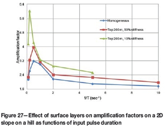
The effect of horizontal layering is examined using a 2D model. As shown in Figure 25, a softer material is assumed to a depth of 200 m below the slope toe. Two cases are studied. In the first case, the softer material has a modulus that is 50% of the original modulus, whereas in the second case, the modulus is 10% of the original value. The results for the slope geometry are shown in Figure 26 and the results for the hill geometry are shown in Figure 27.

 

 

 

 

 

 

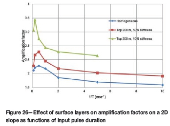
The presence of softer material leads to energy trapping within the narrow layer below the surface, and hence much higher amplification ratios are observed. For the slope geometry, the maximum amplification increases to about 2.7 for the 50% stiffness case, whereas an amplification ratio of 3.6 is observed for the 10% stiffness case. The frequency corresponding to peak amplification also decreases as stiffness decreases.

For the hill geometry, the effect is even more pronounced with an amplification ratio of 4.0 for the 50% stiffness ratio, and 6.0 for the 10% stiffness ratio. As the stiffness contrast increases, the amplification ratio also increases. While it is common to have a thick layer of highly weathered rock or soil above competent rock on natural slopes, open pit slopes are generally excavated in relatively good quality rock and have only a comparatively thin layer of fragmented rock that is still stiffer than highly weathered rock or soils; hence open pit slopes are less susceptible to amplification due to material heterogeneities.

B.2 Effect of vertical layering

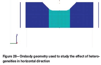
Material heterogeneities can also be present in a horizontal direction (e.g., due to the presence of the orebody). The effect of an orebody is evaluated in this section in 3D where the orebody is assumed to be vertical and intersects the pit walls 100 m above the base of pit as shown in Figure 28. The orebody is assumed to have half the stiffness of country rock. Results are shown in Figure 29.

 

 

 

 

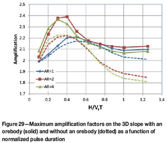
As expected, the presence of the orebody leads to higher amplification ratios than for the homogenous case as energy is trapped within the orebody. one of the important observations is that the increase in amplification ratios is more pronounced for higher aspect ratios than for the circular case, where the increase is negligible. Nonetheless, the peak amplification ratio for the 4:1 case is still 2.4, which is not too high compared to the amplification ratio of 2.0 for the free field base case.