PAPERS OF GENERAL INTEREST

 

Stochastic simulation of the Fox kimberlitic diamond pipe, Ekati mine, Northwest Territories, Canada

 

 

L. Robles-Stefoni^I; R. Dimitrakopoulos^II

^ICOSMO - Stochastic Mine Planning Laboratory
^IIDepartment of Mining and Materials Engineering, McGill University, FDA Building, 3450 University Street, Montreal, Quebec, H3A 2A7, Canada

 

 

---

SYNOPSIS

Multiple-point simulation (MPS) methods have been developed over the last decade as a means of reproducing complex geological patterns while generating stochastic simulations. Some geological spatial configurations are complex, such as the spatial geometries and patterns of diamond-bearing kimberlite pipes and their internal facies controlling diamond quality and distribution.
Two MPS methods were tested for modelling the geology of a diamond pipe located at the Ekati mine, NT, Canada. These are the single normal equation simulation algorithm SNESIM, which captures different patterns from a training image (TI), and the filter simulation algorithm FILTERSIM, which classifies the patterns founded on the TI. Both methods were tested in the stochastic simulation of a four-category geology model: crater, diatreme, xenoliths, and host rock. Soft information about the location of host rock was also used. The validation of the simulation results shows a reasonable reproduction of the geometry and data proportions for all geological units considered; the validation of spatial statistics, however, shows that although simulated realizations from both methods reasonably reproduce the fourth-order spatial statistics of the TI, they do not reproduce well the same spatial statistics of the available data (when this differs from the TI). An interesting observation is that SNESIM better imitated the shape of the pipe, while FILTERSIM yielded a better reproduction of the xenolith bodies.

Keywords: multiple-points simulation methods, SNESIM, FILTERSIM, categorical simulation, cumulants, high-order statistics

---

 

 

Introduction

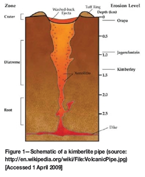
The simulation of geological units poses several technical problems that challenge the capabilities of available geostatistical simulation approaches and their ability to deal with spatial complexity of categorical variables. The spatial geometry of diamond-bearing pipes and their internal facies controlling diamond distributions are a specific and well-known difficult modelling problem. The geometry of a kimberlite pipe is typically like an inverted cone (Figure 1); the wider part is known as the crater and is located near the surface, and the narrower, deeper part is known as the diatreme. Xenolith bodies can also be found inside the pipe. A very important contribution to the geological modelling of the contours of the pipe is the measure of uncertainty about the location of the contact between the kimberlite pipe and the host rock.

 

 

Rombouts (1995) mentioned that a good evaluation of a diamond deposit requires a detailed analysis of the statistical distribution of the number of occurrences, sizes, and values of the diamonds. Applications of stochastic modelling of the geometry of a pipe were developed by Deraisme and Farrow (2003, 2004). In this case, they simulated first the walls of the pipe, and afterwards used a truncation of a Gaussian field to simulate the layered rock categories present inside the domain of the pipe. Deraisme and Field (2006) also implemented pluri-Gaussian simulation as a more complete categorical simulation method for the interior layered zones of a pipe.

Another application of simulation of geometry on a kimberlite pipe can be found in Boisvert et al. (2009). In this application, they built a stochastic simulation of the geometry of a kimberlite pipe conditioned to a piercing point's data-set. The simulation was conducted on the cylindrical space by transforming x-y-z coordinates to θ-r-z (rotation angle, radius, elevation) coordinates. A vertical trend was defined for the radius, as it decreases towards the bottom of the pipe. However, this methodology assumes that the walls of the pipe are smooth and cylindrical, making it hard to use for more complex kimberlite models. A possible inconvenience is that the transformation of the coordinates may lead to an order problem when back-transforming the simulated values. The main drawback of the method is that the wrapping of the rotation angle may not ensure continuity in the points being simulated at each level.

The reproduction of complex geological features present in kimberlite pipes can be addressed with newer multiple-point (MP) methods. MP modelling techniques focus on reproducing the geological patterns and shapes of orebodies; for example, they focus on the reproduction of complex spatial arrangements, such as xenoliths in the diatreme part of a pipe. Other than the MP methods discussed next and applied herein, related methods in the technical literature include those of Daly (2004) and Kolbjornsen etal. (2014), who worked on a multiple-point approach focused on Markov random fields. Tjelmeland and Eidsvik (2004) applied a metropolis algorithm for sampling multimodal distributions. Arpat and Caers (2007) and Honarkhah and Caers (2012) developed computer graphic methods to reproduce patterns in images. Gloaguen and Dimitrakopoulos (2009) implemented a simulation algorithm based on the wavelet decomposition of geophysical data and analogues of the geological model; this method is able to reproduce nonstationary characteristics. This framework was extended to MP simulations for both categorical and continuous variables by Chatterjee et al. (2012) and Chatterjee and Dimitrakopoulos (2012). Mustapha and Dimitrakopoulos (2010) presented high-order simulations based on conditional spatial cumulants.

Multiple-point methods are based on the use of training images (TIs), which are interpretations or analogues of the possible geological patterns that underlie the phenomenon studied. The TIs usually have a regular spatial configuration, which facilitates the inference of spatial patterns and their probability of occurrence. Templates are used for scanning TIs that represent information about a particular geological model. A pattern is a possible configuration of values obtained by scanning the TI with the template. Single normal equation simulation (SNESIM) is a fast MP simulation algorithm developed by Strebelle (2002) as an extension of past approaches (Guardiano and Srivastava, 1993). When using SNESIM, the patterns are saved in a tree-like data structure, together with their conditional proportions. An application of this method to the modelling of a curvilinear iron deposit can be found in Osterholt and Dimitrakopoulos (2007). The latter work reports a known limit of the MP methods, i.e. their inability to always reproduce the two-point spatial relations in the data available, although all statistics of the TI are reproduced. MP methods are TI-driven as opposed to data-driven, and when there are differences between the higher order relations in the data and the TI, the TI characteristics prevail.

Filter-based simulation or FILTERSIM (Zhang et al., 2006; Wu et al., 2008) is a MP simulation method that associates filter scores to patterns. This recent simulation approach groups patterns into classes of patterns. The classification of patterns is made according to a small set of scores per pattern. The score is obtained by applying filter functions to the values at the template nodes. The underlying assumption is that similar patterns will have similar scores. During the pattern simulation, the selection of the class from which the pattern will be retrieved is given by measures of distance and similarity.

In the present study, first, the SNESIM and simulation using filters (FILTERSIM) are revisited. Then, the two methods are used to stochastically simulate lithology categories of the Fox diamond-bearing kimberlitic pipe, located on the Ekati property, Northwest Territories. Finally, the performance of the stochastic outputs from SNESIM and FILTERSIM outputs are compared and validated in terms of the high-order statistics reproduced.

 

A review of multipoint simulation methods

Sequential simulation

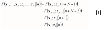
Sequential simulation offers a class of stochastic simulation algorithms (Ripley, 1987). In particular, sequential simulation is also part of the MP simulation algorithms used here. The basic concept consists of modelling and sampling local conditional distribution functions (cdfs) at each node of a grid. The multivariate N-point cdf of a stationary random field can be written as a product of Ν univariate cdfs (Equation [1]),

Conditional simulation using a single normal equation

The following description of a single normal equation follows the one presented in Guardiano and Srivastava (1993). Consider the existence of an unsampled location x₀, and an event A₀ at that location. At each data location there is a data event A_a; a simple data event would be a single datum A_a:[Z(xJ = z_a], and a complex data event would be the whole data-set S(n):[Z(x_a) = z_a, a = 1,.....,n}.

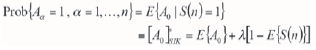
The conditional probability of the event A₀ given the n data events A_a= 1, a = 1,...,n, is equal to the conditional expectation of the indicator random variable A₀.

is the single indicator of the global data

event S(n) = 1 that occurs if, and only if, all elementary data events occur simultaneously, 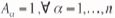Given this relationship, the system of normal equations can be reduced to a single one (Equation [2]):

Equation [3] can be read as a Bayes relationship for conditional probabilities; the result of indicator kriging using a single global data event is equivalent to the Bayes postulate. Equation [3] can be expressed in probability terms:

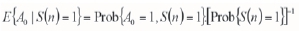
These probabilities can be obtained from real data-sets or TIs by scanning them. In particular, E{A₀.S(n)} is the frequency of occurrence of the joint event, and E{S(n)} is the frequency of occurrence of the global data event.

SNESIM was proposed by Strebelle (2002) and its computational aspects were since revisited and improved (Strebelle and Cavelius, 2014). In the SNESIM algorithm a TI is scanned in order to infer the relative frequency . Each pattern scanned on the TI is saved in a binary search tree together with its conditional probability. Each pattern is saved in the tree, and every pattern is a leaf of the tree. The conditional probability of a particular pattern is calculated by counting the frequency of appearance of the pattern in the TI. The root of the tree contains the simplest search templates, and moving towards the leaves, the template size increases given that more possible configurations are available. The tree is constructed from the TI occurrences, not from the total number of theoretical occurrences.

Afterwards, a simulated value at node x₀is obtained by drawing a realization of A₀using Monte Carlo simulation methods. The sequential simulation rule is implemented such that each simulated value is kept as a data event for subsequent nodes. The global data event will grow by one unit S( n+1); if N nodes are simulated the last node will have a data event of size (n + N - 1). Simplification suggests keeping just the nearest conditioning data events, reducing the number n and complexity of data events. The SNESIM algorithm can be applied only to categorical variables. As an example, when using five categories and a data event of 16 nodes (K = 5 and n = 16), there are up to Kⁿ= 1.5 x 10¹¹ joint realizations of the n data values. This should not be a problem if there is consistency between the hard data and the TI, so the data event is easily found during the scanning of the training image.

SNESIM is reasonable in its computational aspects, as it uses less CPU time by scanning the TI once. The conditional probabilities and the patterns are saved in a data structure; this facilitates the search when performing the simulation without demanding excessive RAM. Computational aspects of SNESIM have recently been revisited and further improved (Strebelle and Cavelius, 2014). One limitation is related to the scope of the studies that can be done using this method, given that it works only using categorical data. Another limitation is that discontinuities or nonstationarity behaviours in the TI will not be reflected in the simulation outputs, unless enough conditioning data is available given that local information is lost when saving patterns in the search tree. Another drawback is that when finding the data event, the hard data locations are moved to the closest node in the search template configuration; however, this induces a screen effect and other close data values could be ignored.

SNESIM algorithm

1. Scan the training image with particular data template t_nof n nodes. Store the patterns along with the cdfs in a search tree. The cdf is calculated using the Bayes relationship. The total number of occurrences of the data event is ( c( d_n)), and the number of times this data event has a central value belonging to class k is defined as (c_k(d_n))

2. Each node on the grid is visited once along a random path. At each node u, obtain the conditioning data event inside the data search neighbourhood W(u), which is a sub-template of x_n. Then find this pattern on the tree, and draw a realization of the central value by sampling from the conditional probability distribution function. The central value is used as hard data for subsequently simulated nodes.

Example of a binary tree

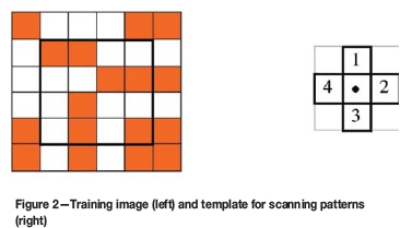
A two rock-phase training image and a squared template of four nodes are shown in Figure 1. The template is used to scan the TI; but only the inner nodes of the TI are used, to ensure that all the nodes in the template are assigned a particular rock value. The construction of the search tree would follow these steps:

1. Use the node located in the centre of the template to count the frequency of coloured versus white nodes located on the inner part of the TI, in this case 4x4 nodes giving a total of 16 (do not count the first and last rows and columns). This gives a distribution of 9 whites and 7 coloured. These frequencies are saved on the head of the search tree

2. Use the template node in the centre and the one in the position 1 to scan the TI. There are two possibilities; node 1 is either white or coloured. If the centre node is white, node 1 is white 4 times and coloured 5 times. If the centre node is coloured, node number one is 6 times white and 1 time coloured

3. Use three nodes in the template to scan the image: centre, node 1, and node 2. Now there are eight total possible combinations. For each possible combination, count how many times it appears in the TI. There is one pattern that does not exist on the TI, so instead of eight we will have just seven possible patterns

4. Use the four nodes to scan the TI (centre, nodes 1, 2, and 3). The total number of possible combinations is 16, but only 10 of the combinations are present in the TI

5. Use the five nodes to scan the TI (centre, nodes 1, 2, 3, and 4). The total number of possible patterns is 32, but only 20 of the combinations appear in the TI.

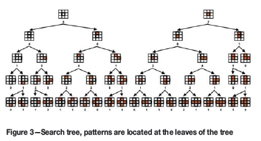
The possible patterns will be the leaves of the search tree, and their frequency of appearance is registered on the tree. Figure 3 shows the final search tree for this small example. It will be noticed that simple configurations are in the root of the tree and the complex ones towards the leaves.

 

 

 

 

Conditional simulation based on filter functions

FILTERSIM is a multiple point simulation algorithm that was introduced by Zhang et al. (2006); it works with both categorical and continuous TIs (it was mostly developed for continuous TIs). The filter simulation consists of three main steps: filter score calculation, pattern classification, and pattern simulation.

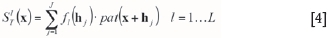
A set of mathematical functions called filters is applied to the TI. The TIs are scanned using a template configuration. Each TI's pattern has a set of filter scores. A template Tj = [x₀;hj, j = 1...J} is a set of J points χ = x₀+ hj j = 1... J described by the origin coordinates x₀and the offset distance h_j. A filter is a set of weights associated with a template Tj. There are L filters functions for a template with J nodes {f_i5(h_j) j = 1... J, l = 1...L}. A training pattern (pat) centred at location x of template Tj has a set of L scores associated that are calculated using Equation [4].

In the case of K categories, the image is divided into K

binary indicators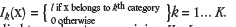

The filters are applied to each category, giving K x L scores for each pattern. A continuous TI is a particular case of a categorical TI with only one category.

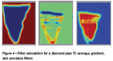
There are three default filters (average, gradient, and curvature) for each axis X - Y - Z. The template size is n_i, for each direction i; the filter node offset is α_i· = -M_i,...,+M_i,· with m_i = (n_i- 1)/2; finally, the filters can be defined as:

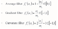
There is a minimum of nine filters scores considering three default filters in 3D; three of which are shown in Figure 4 for the case of a diamond pipe TI. The main aspect of FILTERSIM is the dimension reduction, where a pattern of J nodes is reduced to only K x L scores.

 

 

From this set of scores, the patterns (pat) can be classified and grouped into several pattern classes, called prototype classes prot), which assumes that similar patterns will have similar filter scores. A prototype (prot) is defined as the pointwise average of all the patterns belonging to the prototype class, and it has the same number of nodes as the template (Equation [5]).

The total number of replicates, c, corresponds to the number of patterns extracted from the TI that belong to the specific prototype class.

The categorical prototype is a set of Kproportion maps. A proportion map gives the probability of a category prevailing at template location x_i+ h_j(Equation [6]).

There are two options to classify and group patterns. One is to define arbitrary thresholds in the score space; this is called cross-partition. The other option is called K-mean partition; and it applies clustering techniques in the score space.

Finally, sequential simulation is performed by drawing patterns that honour the data-set. A conditioning data event (dev) is obtained from the neighbouring data using the same template utilized to scan the TI. Hard data is moved into grid nodes for each simulated node x, then the set of scores is calculated for that data event.

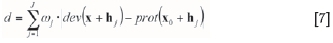
The closest pattern class (prot) is chosen by means of a minimum distance measure d (dev, prot) defined in Equation [7]. The final simulated object is pulled by random selection from the set of patterns belonging to the selected pattern class. Afterwards, the pattern is pasted into the simulation grid and is used as hard data for the next point being simulated. The simulation is made starting from a coarse grid and then continuing with finer grids, helping with the reproduction of large-scale and small-scale features.

The main advantages of this method are related to the speed and computing performance; it is fast since it scans the TI once with a given template size. This algorithm is less demanding on RAM than SNESIM. In particular, the pattern information is represented by a smaller set of filter scores instead of the larger template dimensions; this reduction generates an increase in the speed of the algorithm.

The counterpoint relates to the output simulations, because these will depend strongly on the size of the template being used. Not only will the running times depend on the size of the template; the quality of the simulation will decrease when using large templates, by showing artifacts. On the other hand, a small template can miss some large-scale behaviours of the TI. In summary, a good quality simulation output will require a careful selection of the template size. Also, the selection of the filter functions being used is important; some filters may give redundant information about the TI, for example when the TI is symmetric. Another drawback of this method is the repositioning of the hard data information into grid nodes each time a data event is obtained.

FILTERSIM algorithm

Repeat:

1. Rescale to g^thcoarse grid

2. Calculate scores using rescaled filters

3. Divide (pat)s into (prot)classes

4. Relocate hard conditioning data into grid G^g

5. For (each node u)

a. Extract ( dev) at u

b. Find (prot) class using ô(dev, prot)

c. Sample (prot) class to get (pat)

d. Paste ( pat) to realization

6. End for

7. Ifg* 1, take out hard conditioning data from G^guntil all multi-grids G^ghave been simulated.

 

Case study

Geology of Fox-Ekati kimberlite pipe The Ekati property, located in the Northwest Territories in Canada, is one of the main diamond producers in the world. BHP Billiton has mined diamonds from Ekati since 1998. In 2003, 150 kimberlite pipes had been found, and five of them were being mined: Fox, Panda, Misery, Beartooth, and Koala North. In June, 2002, BHP Billiton reported a total resource of 113 Mt, with an average grade of 1.3 carats per ton (Dyck et al., 2004). Nowicki et al. (2003), reviewed the geology of the five kimberlite pipes that are being mined on the Ekati property.

The shape of the pipes is mainly like an inverted cone (Figure 1); the wider part of the pipe is known as the crater and is located near the surface and the narrower, lower part of the pipe is known as the diatreme. A very important contribution to the geological modelling of the contour of the pipe is the measure of uncertainty about the location of the contact between the kimberlite pipe and the host rock, mainly because all the material inside the pipe is considered as ore and is sent to the processing plant. The mining operations at Ekati are based on open pit designs where the usual mining bench is about 10 to 15 m high; moreover, the host rock quality is good enough to allow for a steep slope angle.

According to Nowicki et al. (2003), the Ekati pipes are composed mainly of volcaniclastic kimberlite material (VK), such as fine- to medium-grained crater sediments, resedimented volcaniclastic kimberlite (RVK) that is ash/mud-rich to olivine-rich, and primary volcaniclastic or pyroclastic kimberlite (PVK).

Fox is the largest orebody, 550 by 630 m in area and 810 m in depth. Fox is situated within the biotite granodiorite of the Koala Batholith. In general, the wall rock contact follows a circular shape and in detail it is irregular and strongly controlled by faults; the wall rocks also include several diabase dykes. Fox pipe has two different phases: an upper flared zone (100-150 m thick) that contains mainly mud-rich resedimented volcaniclastic kimberlite (mRVK) and a lower diatreme-shaped zone filled mainly with tuffisitic kimberlite (TK). The contact between the crater and the diatreme zone is sharp. There are large granodiorite boulders within the TK phase, below the RVK phase, in the lower part of mRVK phase, and sporadically in the tuffisic kimberlite.

Exploratory data analysis

Drill-hole samples contain information about the sample length, the number of diamonds found, and the bulk density. There are 8991 samples with lengths ranging from 0.01 to 821.8 m; on average, samples are 5 m long. Compositing is necessary to regularize the sample length. The maximum number of occurrences of stones is 44, and the average is 7 stones. The average rock density is 2.1 t/m³.

As mining operations are based on open pit designs with a typical bench height of 10 m, this measure is chosen as the composite length. The composites were built respecting the lithological codes in order to have representative samples for each rock category, which is the main objective of this case study. There are 3610 composites samples that have an average length of 9.9 m; the minimum length is 7 m and the maximum 10 m.

The association between the rock categories in the hard data-set (containing 44 rock categories) and the 3D solids interpreting geological zones (crater, diatreme, xenoliths, and host rock) is not straightforward. The crossing of information between lithological codes and rock solids leads to the following classification:

> Granodiorites are associated with the host rock (code 0)

> Resedimented kimberlites, olivine kimberlites, and sands are with the crater solid (code 1)

> Tuffisitic kimberlites and primary kimberlites are associated with the diatreme solid (code 2)

> Breccias are associated with xenoliths (code 3).

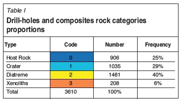
Figure 5 shows a vertical section of the composited drillhole samples classified into the previously mentioned rock categories. Xenoliths are present inside the pipe's crater and also in the diatreme; these bodies are considered to be mainly waste, so their geological modelling is interesting, since their tonnage should be discounted from the total ore reserves. The composites samples, rock type proportions are summarized in Table I.

 

 

 

 

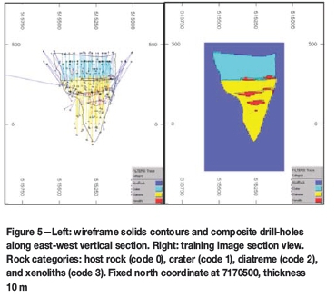
Geologists provided three wireframe solids representing the geological model of Fox kimberlite pipe (Figure 5). The wireframes comprised the wide crater zone near the surface, the narrow diatreme zone at the bottom, and the xenolith bodies inside the pipe. The lentil-shaped circles around the middle zone are xenolith orebodies. These solids are used as base information for the construction of a TI. The TI is a three-dimensional grid with nodes 10x10x10 m apart; which dimensions are 54x63x81. The origin is (XxYxZ): (515060x7170200x-300). Each grid node can have one value among the four phases; each phase has a numeric code: 0 for host rock, 1 for crater, 2 for diatreme, and 3 for xenoliths.

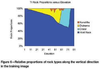
It is interesting to observe how the proportions of the different rock types change along the vertical direction in the TI. From top to bottom, the relative proportions were calculated every 10 m; the graphic with the proportions information is shown in Figure 6. The vertical axis shows the relative proportions of each of the four rock types, and the horizontal axis the elevation. Level 1 is at the bottom of the pipe and level 81 near the surface. The proportion of nodes inside the pipe decreases with increasing depth as the pipe is narrower at the bottom. There are four main xenolith clusters, mostly located between the vertical levels 40 and 65. In Figure 6, the area covered in colour by each rock type can be used to calculate the total tonnage of that particular rock type.

 

 

This TI does not meet the assumption of stationarity because the rock type proportions change considerably along the vertical axis. Also, the patterns do not repeat themselves multiple times. The lack of stationarity can be overcome by adding data in zones where hard data is scarce and there is a strong geological expectation for a given rock type. For example, granite (host rock) would be expected outside the boundaries of the pipe. The use of abundant soft data was proposed to overcome the problem, because the conditioning step should ensure the reproduction of trends and complex patterns.

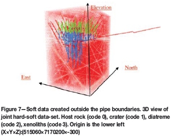
Soft data is added outside the pipe limits in a regular grid of 10x10x10 m. Thus, artificial hard information with rock code 0 is added. The soft data generation process is done using an algorithm that grows a given 3D object. The number of times the object grows is an arbitrary election based on the tolerance to geological uncertainty. In this example, the entire pipe (union of crater and diatreme solids) is used as the 3D object. At each iteration, the pipe grows 10 m along each axis; in particular, this means the closest nodes with code 0 located at the pipe's border become part of the pipe for the next iteration. For this particular case study, the pipe has been grown five times, giving 50 m to allow for geological uncertainty. The nodes outside the last 'bigger' pipe are selected as locations for soft information (host rock). An image of the soft information added outside the boundaries of the pipe is shown in Figure 7.

 

 

Stochastic simulation using SNESIM

The SNESIM algorithm was utilized to obtain a stochastic geology model. The simulation grid size has 54x63x81 nodes located every 10x10x10 m. Soft data is included. The algorithm needs as input the global marginal distribution of the four categories; this was obtained by counting the number of nodes that belong to each category. From a total of 275 562 nodes in the training image grid, 222 090 belong to host rock, 23 434 to crater, 27 598 to diatreme, and 2440 were xenoliths (proportions: 0.806 host rock, 0.085 crater, 0.100 diatreme, and 0.009 xenoliths.).

The RAM requirement and running time are increased by augmenting the number of nodes in the search template, but this will lead to a better reproduction of the patterns existing in the TI. In this case, 80 nodes inside the search template are selected. The election of the search template geometry was isotropic with 50 m (five nodes) in the X, Y, and Z directions.

The 'minimum number of replicates' parameter can be described as the number of times a pattern similar to the data event is present in the TI; the minimum frequency of that given pattern in the search tree. If this number of replicates is met, a simulated pattern will be retrieved from the conditional probability distribution. In this case, the minimum number of replicates is unity; if there is just one replicate of the data event in the search tree this particular pattern will be retrieved with 100% probability. Three multiple grids are chosen to ensure the reproduction of large and small scale pattern continuity.

Ten realizations were generated in order to assess the geological uncertainty. The running time was 5.78 minutes. Figure 8 shows a section view of four realizations obtained. SNESIM realizations respect the main geometric configurations; crater rocks are at the top, diatreme rocks are at the bottom, and xenoliths are inside the pipe; however, the xenoliths are choppy and scattered. The host rock wall is as not as soft as in the TI. The SNESIM algorithm gives a reasonable structural quality of its realizations; however, the quality of the simulations must be measured using highorder statistics.

 

 

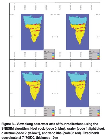
Figure 9 shows the vertical level-by-level proportion curves for each rock category and for every realization. Each level has 54x63 blocks; there are 81 vertical levels. Each block is assigned to one of the four different rock codes.

 

 

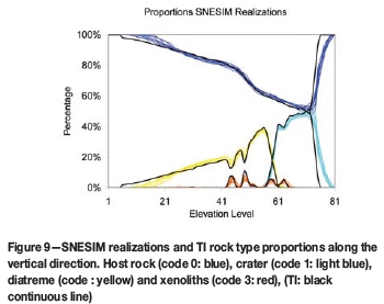
There are ten realizations. Blue lines describe the number of blocks with the host rock code, light blue lines those assigned to the crater, yellow lines the diatreme, and red lines those belonging to the xenoliths. Black lines show the proportions of the rock types in the TI. In general, the realizations respect the proportions of the three main rock categories (crater, diatreme, and host rock); however, the proportions of xenolith rocks are underestimated. The realizations also follow the same level-by-level inflections of the proportion curves. The TI and the realizations curves follow each other closely between the top level (around level 81) and the bottom level (around level 0), where there is more consistent conditioning information.

For the purpose of comparing between the TI and the stochastic realizations, cumulants of fourth order were calculated (Dimitrakopoulos et al., 2009) When a fourth-order cumulant is calculated, three different directions are provided. In this case, top-bottom, east-west, and north-south are chosen. The cumulant of fourth order is a 3D object with different cumulant values at each node. Each node in the cumulant object can be specified by three lags or distances to the origin, defining a search template. The training image and the geological realizations are scanned using this template, generating one cumulant value for one node in the object. Cumulants can be calculated on continuous variables or indicator (0-1) variables (Dimitrakopoulos et al., 2010). Cumulants on the TI can be calculated if we label the crater, diatreme, and xenoliths as code 1 (inside pipe) and the host rock as code 0 (outside pipe). Another cumulant map can be obtained by labelling the xenoliths as code 1 and the crater, diatreme, and host rock as code 0 (outside xenoliths). Figure 10 shows the cumulant 3D objects calculated by scanning the TI multiple times with multiple templates. The cumulant maps provide structural information on the general shape of the kimberlite pipe. Also, cumulants identify the main distances between xenolith bodies along the vertical level and their lentil-shaped structure. The fourth-order cumulant maps on the composite drill-hole samples were also calculated in Figure 11. Although the cumulant object is incomplete since the composite samples are not fully informed on space, nevertheless the main shape of the cumulant object is reproduced.

 

 

 

 

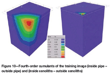
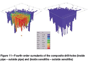
Figure 12 shows the cumulants of fourth order of one realization obtained with SNESIM. The xenolith cumulants show a tail, which differs from the training image. The continuity of the xenolith's bodies in the simulated maps is poor, and the cumulant map reflects this situation.

 

 

Stochastic simulation using FILTERSIM

The categorical version of the FILTERSIM simulation algorithm was used to obtain several conditional realizations, which produced a model of the geological uncertainty. The most relevant parameters used are detailed as follows.

The template size strongly influences the running time of the algorithm. The running time does not follow a linear behaviour when increasing the template size; this can be explained as follows. FILTERSIM consist of three main calculation parts - filter calculation for the training image; pattern classification, which may be dominant when clustering into prototypes; and pattern simulation, which may be dominant when finding the distance between the data event and different prototypes.

A larger template is conducive to finding fewer patterns while scanning the TI; then, the minimum number of expected replicates should be reduced. With a larger template it is harder to find a data event; then the algorithm starts doing unconditional simulation, and the reproduction of geology becomes poorer. A smaller template produces a more accurate reproduction of the TI, more replicates for each pattern, and then a better subdivision, but the running time increases. While decreasing the template does not mean increasing the running time further; some smaller templates reach simplicity in the patterns found, which decreases the running time. The extreme case is a template size of a single node. In the case of a binary variable there will be two main prototypes classes, 0 and 1; however, the quality of the realizations becomes useless as they show lack of continuity and, in the extreme case, a pure nugget effect.

Finally, the template size 5x5x7 was used for obtaining 10 realizations in the four-phase case study. The patch size should ideally be just one node, to be pasted into the simulated grid, but in this case running time will increase, and this can also lead to lack of reproduction of small-scale patterns. The patch size chosen is 3x3x5, which is small enough to ensure the absence of artefacts and large enough to have a reasonable running time.

The number of multiple grids used helps the reproduction of largescale and small-scale patterns; however, it makes the running time longer. In this case study, two multiple grids would be chosen. The minimum number of replicates is the pattern prototype splitting criteria, to split a parent class into child classes. Only those parent patterns with more than 10 occurrences are further split into child classes. In this case study, cross-partition is used, selecting four divisions as a parent splitting criteria at each filter score, and two as secondary splitting or child partitions. The data weights for hard, patch and other are 0.5, 0.3, and 0.2, respectively.

An image with an output of four realizations is shown in Figure 13. From a purely visual inspection, the realizations seem to follow the main structural features of the pipe, generating xenolith bodies only inside the pipe boundaries and following closely the pipe's cone shape. Some realizations lose continuity in the crater phase near the top and in the diatreme phase at the bottom.

 

 

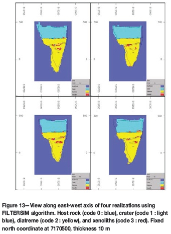
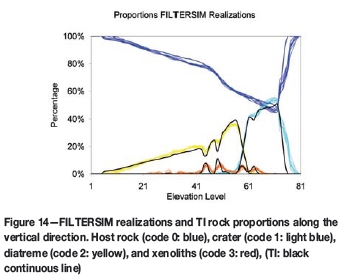
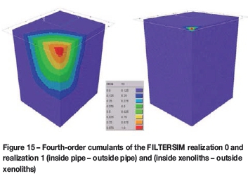
Figure 14 shows the vertical level-by-level proportion curves for each rock category and for every FILTERSIM realization. In general, the realizations respect the proportions of the three main rock categories (crater, diatreme, and host rock). The TI and the realizations curves follow each other closely between the top level (around level 81) and the bottom level (around level 0), where there is more consistent conditioning information. However, the proportions of xenolith rocks are underestimated; also, the realizations do not follow the TI xenolith curve tightly. Cumulants of fourth order of the FILTERSIM realizations are shown in Figure 15. The xenoliths cumulants appear to follow the TI cumulants better than SNESIM.

 

 

 

 

Comparison between MPS methods

Running time

The FILTERSIM running time is 16 807 529 ms (4.67 hours); which is large in comparison to the SNESIM simulation (346 725 ms (0.1 hours). This can be explained mainly by the fact that the set of parameters chosen for FILTERSIM was demanding. The FILTERSIM algorithm requires less RAM than SNESIM; in consequence, it takes a longer running time. The SNESIM algorithm is faster than FILTERSIM for the same structural quality of its realizations. This gives a major advantage of SNESIM compared with FILTERSIM; the same good simulation outcome can be obtained for less than 10% of the running time.

Relative errors with respect to Tl

In order to compare the SNESIM and FILTERSIM realizations with the TI, the global relative error was calculated using Equation [8].

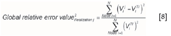
where Ν= 275562 is the total number of nodes in the TI. The value of the cumulant of the stochastic realization j at node i is V^J_iis , and the value of the cumulant of the TI at node i is v_i^TI. There is one global error for each stochastic realization. As there are ten realizations, ten relative error values are generated, one for each cumulant map calculation (inside pipe and inside xenolith cases). The relative error between the cumulant map calculated on the composites and the TI was also calculated.

The summary of these calculations is shown in Table II. The total sum of the squared values of the is 6085.59 for the inside/outside pipe cumulant map; and, 18.04 for the inside/outside xenolith cumulant map. Relative errors in the reproduction of the cumulants of the wall of the pipe fluctuate around 1%; this means that the stochastic simulation algorithms reproduce well the shape of the wall of the pipe provided by the training image. Relative errors fluctuate around 25% for the reproduction of the fourth-order cumulants of the xenolith bodies. Relative errors are much higher in the reproduction of the cumulant values of the xenolith orebodies than in the reproduction of the cumulants of the pipe wall. There is a difference of 26.85% between the composites and the TI. The composites' cumulants follow roughly the same shape of the cumulants calculated on the TI. The cumulant maps of the composite, as well as the training image and the realizations, were re-scaled. Given that the cumulants are used on an indicator variable, they represent mainly geometric features of the map, so the re-scaling does not affect the error calculation because the cumulants are invariant to additional constants; moreover, it helps to clarify the analysis of the errors. All of the cumulant maps were re-scaled to a [0,1] interval, so the comparison between the cumulant maps of the stochastic images, the TI, and the composites is more comprehensible.

 

 

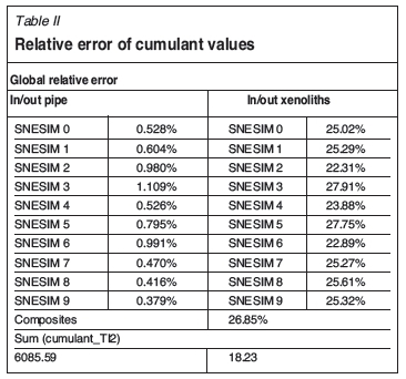
With the purpose of validating FILTERSIM realizations against the TI, the global relative error was calculated using Equation [8]. There are ten realizations per simulation method, and ten relative error values are obtained for each cumulant map calculation (inside pipe and inside xenolith cases). The summary of these calculations are shown in Table III. The relative errors in the reproduction of the cumulants of the wall of the pipe fluctuate around 2% for FILTERSIM. The FILTERSIM realizations' errors for the xenolith maps fluctuate around 15%.

 

 

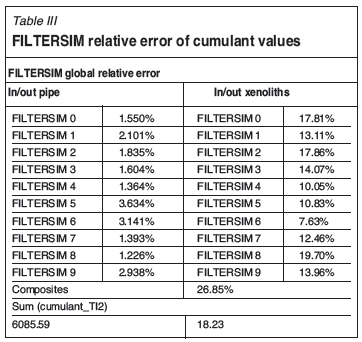
Relative errors are much higher in the reproduction of the cumulant values of the xenolith orebodies than in the reproduction of the cumulants of the pipe wall. FILTERSIM provides better results than SNESIM for the reproduction of the continuity of the xenolith bodies because it simulates patterns; however, the high relative errors reflect the deficiency of both methods in reproducing the high-order statistics when simulating small or medium objects distributed in the geological domain.

Relative errors with respect to composites

The reproduction of the high-order statistics of the composites was analysed by calculating the global relative error with respect to the composite cumulant map. However, since the composite cumulant map is incomplete with respect to the other cumulant maps, only the set of nodes informed on both maps (composite cumulant map versus TI or realizations cumulant maps) contribute to the error calculation. These nodes are called fully informed nodes. Equation [9] is used to obtain the global relative error.

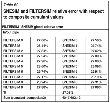
where N = 22945 is the number of fully informed nodes. The global relative errors are shown in Table IV. The total sum 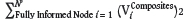for the inside/outside pipe cumulant map. The inside/outside xenolith cumulant global relative error was not calculated since the xenoliths composite cumulant map is poorly informed, and the relative errors do not provide useful information. FILTERSIM errors fluctuate around 27.3% and SNESIM around 27.5%. FILTERSIM reproduces the composites values slightly better. However, both stochastic methods give a poor reproduction of the high-order statistics of the composites.

 

 

The FILTERSIM method uses only a set of linear filters to classify complex geological patterns; then, it may not possible to reproduce nonlinear spatial correlations, i.e. high-order spatial cumulants, of the TI from the simulated images. Furthermore, it is difficult to reproduce the high-order spatial nonlinear cumulants of complex geologic structures using SNESIM, which is based on the calculation of only one linear high-order moment.

 

Conclusions

SNESIM and FILTERSIM were used for the stochastic simulation of geology on the Fox kimberlite pipe. Four categories were used to simplify the geological model: crater, diatreme, xenoliths, and host rock. The training image (TI) provided by the geologist was not stationary. The generation of soft conditioning information outside the boundaries of the pipe (host rock code) was necessary to obtain a good reproduction of the shape of the pipe. SNESIM simulation is much faster than FILTERSIM. Both methods reasonably reproduce the main proportions of the main rock categories (crater, diatreme, and host rock); however, both methods underestimate the xenolith proportions. Fourth-order cumulants were calculated using three main lag directions: top-bottom, east-west, and north-south. Cumulants were calculated on the TI, the composites and the stochastic realizations obtained from SNESIM and FILTERSIM methods. The binary variables chosen for the cumulant calculation are divided into two different rock grouping configurations (inside/outside pipe and inside/outside xenoliths). The inside/outside pipe cumulants show the shape of the pipe, and the inside/outside xenoliths show the vertical distances between the lentil-shaped xenolith bodies. The global relative error was calculated between the cumulant maps of the TI and the stochastic realizations. As the errors of the inside/outside pipe are relatively small, it can be concluded that both methods provide a good reproduction of the training pipe's shape; larger errors are obtained when comparing the inside/outside xenoliths cumulants, indicating that SNESIM and FILTERSIM algorithms perform worse in the reproduction of the xenolith bodies than in the reproduction of the walls of the pipe. SNESIM reproduced the pipe's shape better than FILTERSIM; however, FILTERSIM reproduced the xenolith bodies better than SNESIM.

The assessment of the reproduction of high-order spatial statistics (fourth-order spatial cumulants) by the simulated realizations from the two MPS methods shows that while the realizations tend to reproduce the high-order statistics of the TI, they do not reproduce those of the available data, which in this case study are different to those of the TI. Other methods that may improve this are currently being investigated.

 

Acknowledgements

The work in this paper was funded from NSERC CDR Grant 335696 and BHP Billiton, as well NSERC Discovery Grant 239019 and McGill's COSMO Lab. Thanks are in order to BHP Billiton Diamonds and, in particular, Darren Dyck, Barros Nicolau, and Peter Oshust for their support, collaboration, data from Ekati mine, and technical comments.

 

References

Arpat, G.B. and Caers, J. 2007. Conditional simulation with patterns. Mathematical Geology, vol. 39, no. 2. pp.177-203.         [ Links ]

Chatterjee, S., Dimitrakopoulos, R., and Mustafa, H. 2012. Dimensional reduction of pattern-based simulation using wavelet analysis. Mathematical Geosciences, vol. 44. pp. 343-374.         [ Links ]

Chatterjee, S. and Dimitrakopoulos, R. 2012. Multi-scale stochastic simulation with wavelet-based approach. Computers and Geosciences, vol. 45. pp.177-189.         [ Links ]

Daly, C. 2004. High order models using entropy, Markov random fields and sequential simulation. Geostatistics Banff2004. Leuangthong, O. and Deutsch, C. (eds). Springer, Dordrecht, vol. 2. pp. 215-224.         [ Links ]

Dimitrakopoulos, R., Mustapha, H., and Gloaguen, E. 2010. High-order statistics of spatial random fields: Exploring spatial cumulants for modeling complex, non-Gaussian and non-linear phenomena. Mathematical Geosciences, vol. 42, no. 1. 6 pp. 5-97.         [ Links ]

Dyck, D., Oshurst, P., Carlson, J., Nowicki, T., and Mullins, M. 2004. Effective resource estimates for primary diamond deposits from the Ekati Diamond MineTM, Canada. Lithos, vol. 76, no. 1-4. pp. 317-335.         [ Links ]

Gloaguen, E. and Dimitrakopoulos, R. 2009. Two-dimensional conditional simulations based on the wavelet decomposition of training images. Mathematical Geosciences, vol. 41, no. 6. pp. 679-701.         [ Links ]

Guardiano, F.B. and Srivastava, R.M. 1993. Multivariate geostatistics: beyond bivariate moments. Geostatistics Troia 1992. Proceedings of the Fourth International Geostatistics Congress, vol. 1. Soares, A. (ed.). (Kluwer Academic Publishers, Dordrecht, The Netherlands. pp. 133-144.         [ Links ]

Honarkhah, M. and Caers, J. 2012. Direct pattern-based simulation of non-stationary geostatistical models. Mathematical Geosciences, vol. 44, no. 6. pp. 651-672.         [ Links ]

KOLBJ0RNSEN, O., Stien, M., Kj0nsberg, H., Fjellvoll, B., and Abrahamsen, P. 2014. Using multiple grids in Markov mesh facies modeling. Mathematical Geosciences, vol. 46, no. 2. pp. 205-225.         [ Links ]

Mustapha, H. and Dimitrakopoulos, R. 2010. High-order stochastic simulations for complex non-Gaussian and non-linear geological patterns. Mathematical Geosciences, vol. 42, no. 5. pp. 455-473.         [ Links ]

Nowicki, T., Crawford, B., Dyck, D., Carlson, J., McElroy, R., Oshust, P., and Helmstaedt H. 2003. The geology of kimberlite pipes of the Ekati property, Northwest Territories, Canada. Lithos, vol. 76. pp. 1-27.         [ Links ]

Osterholt, V. and Dimitrakopoulos, R. 2007. Simulation of orebody geology with multiple-point geostatistics - application at Yandi channel iron ore deposit, WA, and implications for resource uncertainty. Orebody Modelling and Strategic Mine Planning, 2nd edn. Dimitrakopoulos, R. (ed.). Spectrum Series 14, Australasian Institute of Mining and Metallurgy. pp. 51-58.         [ Links ]

Ripley, B. 1987. Stochastic Simulation. Wiley, New York.         [ Links ]

Rosenblatt, M. 1985. Stationary Sequences and Random Fields. Birkhâuser, Boston. 285 pp.         [ Links ]

Strebelle, S. 2002. Conditional simulation of complex geological structures using multiplepoint statistics. Mathematical Geology, vol. 34. pp. 1-22.         [ Links ]

Strebelle, S. and Zhang, T. 2005. Non-stationary multiple-point geostatistical models. Geostatistics Banff2004. Leuangthong, O. and Deutsch, C. (eds.). Part 1. Springer, Dordrecht. pp. 235-244.         [ Links ]

Strebelle, S. and Cavelius, C. 2014, Solving speed and memory issues in multiple-point statistics simulation program SNESIM. Mathematical Geosciences, vol. 46, no. 2. pp. 171-186        [ Links ]

Tjelmeland, H. and Eidsvik, J. 2004. On the use of local optimisations within Metropolis-Hastings updates. Journal of the Royal Statistical Society, Series B, vol. 66. pp. 411-427.         [ Links ]

Wu, J., Boucher, A., and Zhang, T. 2008. A SGeMS code for pattern simulation of continuous and categorical variables: FILTERSIM. Computers and Geosciences, vol. 34, no. 12. pp.1863-1876.         [ Links ]

Zhang, T., Switzer, P. and Journel, A. 2006. Filter-based classification of training image patterns for spatial simulation. Mathematical Geology, vol. 38, no. 1. pp. 63-80.         [ Links ]

 

 

Appendix

Experimental calculation ofcumulants

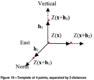
The experimental calculation of cumulants is detailed according to Dimitrakopoulos et al. (2010). A template

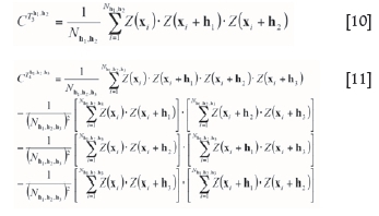
T_n^h₊¹₁^,h2,...,hnis defined as a set of n points separated from the point x by distances h₁,h₂,...,h_n. Every vector h is defined by a lag distance h_i, a direction vector d_iand a supportive angle a_i. An example of a four-point template is shown in Figure 16, which shows three vector distances {h₁^North,h₂^East,h^Vertical,}. The experimental calculation of the third- and fourth-order cumulants are based on average summations in (10) and (11). In this case, N_h1,h2and N_h1,h2,h3 are the number of elements of each template T₃^h1,h2and T₄ h1,h2,h3

 

 

 

When a fourth-order cumulant is calculated, three different directions are provided. In this case, top-bottom, east-west, and north-south are chosen. The cumulant of fourth order is a 3D object with different cumulant values at each node. Each node in the cumulant object can be specified by three lags or distances to the origin, defining a search template. The training image and the geological realizations are scanned using this template, generating one cumulant value for one node in the object.