PAPERS OF GENERAL INTEREST

 

Testing for heterogeneity in complex mining environments

 

 

J.O. Claassen

Department of Geology, University of the Free State, Bloemfontein

 

 

---

SYNOPSIS

Homogeneous populations are required to perform descriptive, probabilistic, and inference statistics and to support stable, predictable mining operations. The geological and downstream processing environments are, however, highly heterogeneous. The complex nature of mining environments requires means to identify and define multi-population environments that could affect the performance of mining value chains. A study performed at several operating mines suggests that the impact of heterogeneous or variable geological, mining, and plant processing environments on overall mining value chain performance may not be a key focus area at these operations. This was illustrated through the use of basic and spatial statistics, which included the log-probability plot, a modified range equation, and chronovariography. The findings reflect high relative variability in the geological and processing environments studied and mining operators' inability to effectively deal with the sources and consequences of variability. The study suggests that a focus on heterogeneity in complex mining operations may significantly enhance overall mining performance.

Keywords: heterogeneity, mining variability, variography, chronovariography

---

 

 

Introduction

Heterogeneity and why it matters

Heterogeneity refers to a state or quality of being variable/diverse and comprising different non-compatible elements or parts. In statistical terms a heterogeneous population can refer to a population comprising different non-compatible sub-populations or a multi-population environment. The latter is commonly found in natural environments such as geological environments (Bardossy and Fodor, 2001). The inherent heterogeneity of complex geological environments is also referred to as spatial heterogeneity. Heterogeneity or variability, however, also occurs over time at mining operations. A case in point is variable ore composition on a conveyance system feeding a processing plant or product stockpile.

Heterogeneity associated with the mining environment can significantly influence key aspects of day-to-day mining operations such as sampling, the use of descriptive, probabilistic, and inference calculations, and an operation's ability to manage and control the mining value chain as a whole.

The sampling regime

The data generated from sampling campaigns forms the basis of nearly all decision-making at the operational, tactical, and strategic levels. As such, it can be argued that the quantity, quality, and correct use of sampling data greatly influence the sustainability of a mining operation.

As far as sampling of heterogeneous environments is concerned, an attempt should be made to capture the variability (both spatial and in time) in all key value chain performance drivers through representative or random sampling. According to the theory of sampling developed by Pierre Gy (1983), sampling errors are induced mainly by high levels of heterogeneity of the population being sampled.

Use of descriptive, probabilistic, and inference statistics

Descriptive statistics are used on a daily basis in mining operations to calculate values such as the average, median, range, and standard deviation of a known data-set. Probabilistic and inference statistics are less frequently employed. Probabilistic statistics (based on probability theory) are used to determine the likelihood or degree of certainty/uncertainty of outcomes drawn from a known population, i.e. if the population is known, what can be deduced from the samples taken from it?

Inference statistics are used to describe an unknown population if everything about the sample is known (random sampling required). Inference statistics involve tests of hypotheses, confidence intervals, and regression.

It should be noted that the existence of a homogeneous population, combined with representative random samples drawn from the population, forms the basis of these calculations as illustrated in Figure 1. This implies that:

 

 

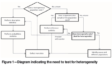
> The application of descriptive, probabilistic, and inference statistical calculations is suspect unless applied to a homogeneous data-set, e.g. calculation of an average value to describe a population is of little value unless it is known that the population is homogeneous

> The geoscientist should test whether heterogeneity exists in a population or sample before proceeding with data analysis, simulation, and graphic presentation of data. This directly affects the accuracy of geological, mining, and financial models and the effectiveness of the reconciliation process, among other things.

If the geoscientist is not aware of this fact, then mathematical blending or integration of non-compatible data (in a multi-population data-set) can lead to a misrepresentation of reality and incorrect decision-making at all levels in the organization, as discussed in more detail in ensuing paragraphs.

Mining value chain management

The mining value chain can be viewed as a complex integrated system. Resources, activities, equipment, and processes are dependent on each other, and the effects of disturbances that occur ripple up- and downstream through the production chain. Forrester (1958), Fowler (1999), Towill (1996), and Wikner et al. (1991) reported that ripple effects are amplified as they move away from the source up or down the value chain, with a significant impact on the performance of the system as a whole due to the destabilizing effect, as illustrated in Figure 2.

 

 

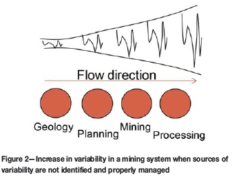
The integrated nature of the mining value chain combined with a heterogeneous geological environment characterized by spatial variability can therefore have a significant impact on the performance of mining operations, i.e. variability leads to poor synchronization of activities and a misalignment between ore characteristics and plant/equipment settings, for example. This implies that if heterogeneity and the sources of variability are not identified and addressed, then the compounding effects (increase in variability when moving away from the source of variability) can completely destabilize a system (lead to stop-start operations) and have a detrimental impact on its overall performance (product volumes, product quality, and cost).

In conclusion, it can be argued that it is essential for mining professionals generating and working with data to utilize means to identify and assist with managing the sources of heterogeneity, as discussed in the ensuing paragraphs.

Means to detect and define heterogeneity

The study, performed at different mining operations, aims to demonstrate how simple statistics can be employed to test for and define heterogeneity. Specific attention is given to the application of a log-probability plot, a modified range equation, and chronovariography.

The study also discusses how information gathered from these basic statistical exercises can be used to improve management of the impact of heterogeneity and the risks associated with it.

The log-probability plot

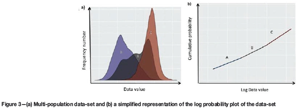
A probability plot is used to indicate deviations from a bell-shaped or normal distribution. It can therefore depict multiple populations or data mixtures through changes in the slope of the graph, as shown in Figure 3b. The x-axis is scaled logarithmically in order to obtain a straight line graph in the case where data is naturally skewed, which is often the case with geological data.

Modified range equation

The 'spread' or range of values in a distribution can be used to indicate heterogeneity or variability. The range equation (Equation [1]) was modified to Equation [2] and applied to daily production data in the study.

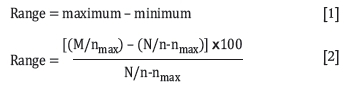
where

M/n_max = Average of daily maximum production values = average of the top 10% values

N/n-nmax = Average of the rest of the values (values including or excluding zero values)

Equation [2] can be used as an indicator not only of variability in, for example, daily production results but also of the improvement potential of a system. In many cases zero values are encountered in the production results of mining operations due, for example, to planned maintenance interventions. If a more realistic improvement potential of a system needs to be calculated, these values can be omitted.

The challenge involved with using an equation such as Equation [2] is to ascertain which benchmark value can be used to evaluate results. In this study a value of 15% was assumed to be reasonable for stable operations, i.e. the maximum values will not differ more than 15% from the rest of the values. More research needs to be conducted to establish what benchmark value is acceptable given the different levels of complexity and variable processing conditions associated with different mining environments.

When Equation [2] is used to calculate variability in sequential steps in the mining value chain, e.g. from blasting to loading, hauling, processing, and product logistics for a variable such as the amount (tons) of material processed, a graphical representation of variability and the operation's ability to manage the sources of variability is generated, as shown later in the paper. The effect of disturbances running through the mining value chain, as alluded to earlier and depicted in Figure 2, can be illustrated using Equation [2].

Variography

Variography has become a frequently employed tool in the geotechnical environment since the work of Krige (1951) and Matheron (1960) that formalized the development and use of variography in spatial estimations. Equation [3] is used to calculate a variogram plot from which a variogram/kriging equation is deduced. The latter is then used for kriging to estimate the spatial distribution of a variable.

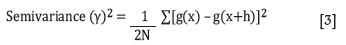
Equation [3] calculates the similarity or homogeneity of values at different pre-set distances (lags) apart; the semivariance is calculated as a function of the differences between distance pairs (g(x) - g(x+h)) and plotted as a semivariogram as shown in Figure 4.

 

 

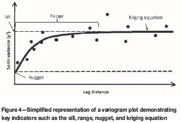
Key indicators defining the variogram include the sill, nugget, and range.

> Sill-Indicates the population variance or total variance in the system as well as the point where data correlates. The sill can be fitted as the total population variance or manually fitted to the semivariogram plot. The latter requires vast experience and knowledge of statistics and the geological environment that is studied

> Nugget-The semivariance at lag distance = 0 reflects the inherent variability in the data as a result of the presence of large grains/nuggets of minerals typically encountered in precious metals and diamond operations. When a nugget value is encountered in more homogenous stratiform deposits or in process streams (chronovariography), it represents sampling, segregation, preparation, and analytical errors. The nugget value can be expressed as a percentage of the total/sill variance

> Range-The range or range of influence represents the point beyond which there is limited correlation between data points. It therefore indicates the maximum 'allowable' frequency of sampling to capture the variability in the variable being studied.

Chronovariography is based on the same principles as variography, except that the semivariance of a variable is calculated as a function of time-pairs and not distance-pairs, as illustrated in the following section. Gy, a metallurgist, developed 'chronostatistics' during the 1950s in order to illustrate the correlations between samples in a time series or product stream (Pitard, 1993, 2006). The development and use of chronovariograms to control a variable in process streams are discussed by Minnitt and Pitard (2008) in detail. The authors illustrate how other key indicators of a chronovariogram, which include the random variability (variance at time = 0 or nugget in variography), total process variability (variability at the first time lag), process variability (the difference between random variability and total process variability), and the cyclical variability (non-random variability at the first sill or semi-sill) can be used to manage variability in process streams as discussed in more detail in the next section.

Other statistical options

Other statistical tools that assists with the quantification and management of variability/heterogeneity not discussed in this paper include chi-square and R charts (Duncan, 1956; Harris and Ross, 1991; Costa and Rahim, 2004; Woodall and Spitzner, 2004). These charts have been extensively used with great success for statistical quality control in the manufacturing and chemical industries.

 

Results and discussion

Basic and spatial statistics are frequently used in geoscience departments to scrutinize geological data, e.g. to identify outliers, define the skewness of populations, and estimate unknown values. However, there is reason to believe that the use of statistical values and graphs to assist with the understanding and management of the impact of heterogeneity on the performance of the mining value chain as a whole is not that common.

The log-probability plot

One of the first activities generally performed when dealing with geological data is to generate a log-probability plot. This is often preceded by a summary of the descriptive statistics and a histogram plot of the data.

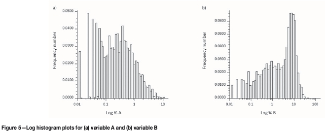
A study was performed on a mineral deposit hosting two mineral entities. Histogram plots of the respective grade distributions for minerals A and B are included in Figure 5 and the log-probability plots in Figure 6.

It is evident from Figures 5 and 6 that the grade distribution of mineral B exhibit at least two distinctive populations, i.e. it is heterogeneous in terms of grade. Care should therefore be taken when applying descriptive statistics. An average grade for mineral B can be calculated to determine the overall in situ metal content associated with mineral B for resource and reserve estimation and reporting purposes. It is, however, essential for the geoscientist to establish the cause(s) of the multi-population data-set (Claassen, 2013) for mineral B prior to estimating product recovery and final product volumes. This stems from the possibility that mineral B associated with populations 1 and 2 (Figure 6b) could behave differently in downstream processing as a result of differences in ore morphology (texture, mineral associations, impurity levels, etc.) and/or orebody morphology (dip, faulting, roof and floor conditions, etc.), which can contribute towards dilution during mining.

In this case an average grade for mineral B was calculated and used in the mine and business plan. ROM grade, mining extraction, recovery, and product quality targets for ROM and final product were seldom met as the plan mostly over- or underestimated the grade of and processing efficiencies for mineral B, depending on which area the operator was mining in at the time. This in turn destabilized the operation and rendered its performance less predictable.

This principle can also be applied to cases where not only chemical grade, but also physical characteristics of the ore and host rock, vary spatially to the extent that different populations are clearly distinguishable. Examples include variability in:

> Hardness, affecting crushing and milling performance and ultimately the liberation potential of the system

> Near-dense material, affecting dense medium separation efficiency, product recovery, and quality

> The level of intergrowth affecting liberation size, which could result in a scenario where ore from different areas is over- or under-milled when blended and simultaneously processed. This in turn has a detrimental effect on product yield and quality.

Claassen (2015) indicated that few southern African mining operators link variable geological environments with processing capability in day-to-day operations, as further demonstrated by this example. The spatial distribution of relevant chemical and physical characteristics of ore and waste, as well as their impact on downstream processing performance, must be understood and correctly included in models and plans.

Modified range equation

Equation [2] was used to study the presence of variability in process streams and the improvement potential at five mines operating in different commodities. Figure 7 summarizes the results obtained for the production rate variability in mining, plant feed (from ROM stockpiles), and plant production for six consecutive months in each case. All the mines utilized a ROM buffer stockpile to improve plant and system performance at the time of the study.

 

 

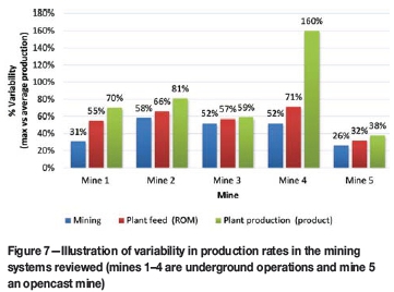
Figure 7 illustrates significant levels of variability (>>15%) at all the operations evaluated, and also an increase in variability in downstream operations (also refer to Figure 2). Table I summarizes the main causes of variability found at these operations.

The results presented in Figure 7 and Table I probably indicates that a focus on heterogeneity and its impact on downstream processing performance does not exist at the operations evaluated, or alternatively that the mines are not successfully dealing with high levels of variability in the geological, mining, and plant environments.

The consequences of the variability observed at these operations include unstable and unpredictable operations, difficulty in estimating realistic production targets for operational and business plans, production targets being seldom met in most cases, operations being mostly in 'fire-fighting' mode, and poor financial performance.

Chronovariography

Heterogeneous geological environments often cause variable processing performance as alluded to earlier. Chronovariograms of plant feed and product streams can indicate the presence and level of variability in these streams and supply very useful information to improve overall process performance, as discussed in the following paragraphs.

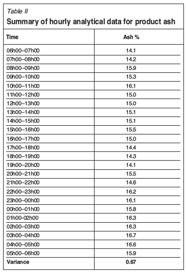
The feed and product streams of five coal processing plants were sampled at hourly intervals and analysed for ash content. To illustrate how a chronovariogram is compiled and used, the product stream data of one of these plants is firstly scrutinized (refer to Tables II and III and Figure 8). This is followed by a chronostatistical analysis of the plant feed variability of four coal processing plants.

 

 

 

 

 

 

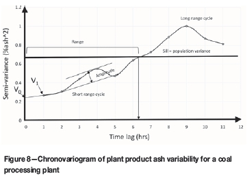
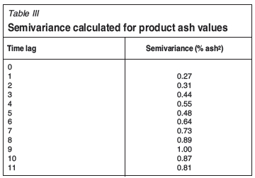
The chronovariogram illustrated in Figure 8 contains the following key variability indicators:

> Sill-the total variance of the data-set was calculated at 0.67% ash²

> Random variability or fundamental error [V₀]-the semivariance at time = 0 represents the sampling, preparation, and analytical error associated with the data-set. In this case it is equal to 0.22% ash² or 0.22/0.67 = 32.8% of the total variance. V₀is obtained by extrapolating the chronovariogram to time = 0. Generally a fundamental error associated with sampling, preparation, and analysis of 10% is assumed to be acceptable. The high value of nearly 33% implies that an effort should be made to investigate these steps to establish what factors contribute towards this error

> Total process variability [V1]-the semivariance at the first time lag represents the sum of the random variability and the variability associated with processing. It is assumed that very little variability is contributed towards total process variability by the material on the conveyor belt within one time-lag. This assumption should be validated for very complex environments. In this case V1 = 0.27% ash² or 0.27/0.67 = 40.3% of the total variance

> Process variability [V1- V₀]- The difference between the total process variability and the random variability is 0.06 ash² or 0.06/0.67 = 9.0% of the total variance

> Cyclical variability [V_c]-the cyclical variance represents the variance at the first or short range cycle, which amounts to V_c= 0.5 χ amplitude = 0.5 χ 0.14 = 0.07% ash² or 0.07/0.67 = 10.4% of the total variance. Mining operations often exhibit cyclical events increasing variability in the system. These events include shift changes, resetting of equipment set-points, changes in equipment performance over time, etc. The short-range cycle visible in this example was a result of changes made in the RD set-points of the plant's dense medium cyclones. In this example, the long-range cycle (9-12 hours) was linked to mining moving from one mining area to another, i.e. a change in the plant feed quality

> Range (hours)- the range deduced from the chronovariogram in this instance is about 6.3 hours. The range indicates the optimal frequency of sampling required to adequately capture short-range variability in the stream. It can therefore be used to optimize plant sampling regimes based on the inherent variability in the system (material being processed as well as the system/process variability) instead of just sampling based on a time or mass setting.

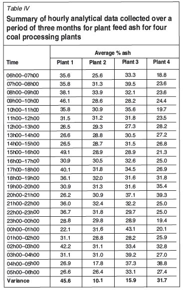
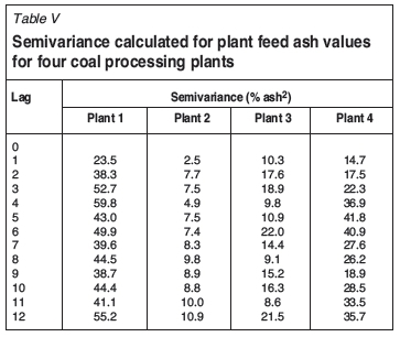
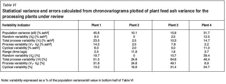
The same approach was followed to study the variability in plant feed quality for four different coal processing plants. The data used was collected over a period of three consecutive months. The data and semivariances calculated from the data are summarized in Tables IV and V, respectively. The values for the chronovariogram variability indicators were obtained from Figure 9 and are summarized in Table VI.

 

 

 

 

 

 

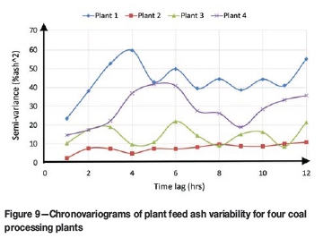
From Table VI the following findings should be highlighted:

> Sill-the total variance in plant feed ash is high for plants 1 and 4 at 45.6% ash² and 31.7% ash², respectively. For plant 1 the random variability contributed about 20% and process variability about 32% of the total sill value. Random variability (39.4%) and cyclical variability (34.7%) are the biggest contributors to variability in the plant feed ash to plant 4

> Random variability [V0]-the relatively high random variability for plants 1, 3, and 4 is probability associated with sampling, preparation, and analysis errors as discussed earlier

> Process variability [V₁ - V₀]-the feed ash variance for plants 1, 2, and 3 exhibits high upstream process variability. In this case the variability was induced during mining operations, mainly as a result of highly variable geological environments and the inability to adjust to mining condition

> Cyclical variability [V_c]-the feed to plants 3 and 4 suffered from cyclical variability induced in upstream operations. It was established that the cyclic events related to mining frequently moving to different mining areas with different conditions and ore quality, i.e. about 5-hourly and 8-hourly cycles for plants 3 and 4, respectively

> Range (hours)-the results indicate that significant increases in short-range variability from the first to second time lag (excluding plant 4) exist. Process and cyclical variability contributed the most towards these increases. In order to enable upstream functions to timeously manage the causes of variability, the frequency of reporting analysis should probably be increased. The total cycle time for sampling, preparation, analysis and reporting should be reduced to between 2 and 3 hours for the plants evaluated. In all the cases the total cycle time for sampling, preparation, analysis and reporting was between 4 and 5 hours.

 

Conclusions

Mining environments are heterogeneous or variable by nature. This variability directly impacts the use of descriptive, probabilistic, and inference statistics as well as an operation's ability to create a stable and predictable business environment.

Descriptive, probabilistic, and inference statistics are applied on the premise that a well-known homogeneous population or representative sample of the population exist. For multi-population distributions, these statistical calculations should be approached with caution. A case in point is the inappropriate averaging or 'mathematical blending' of grade values in a multi-grade deposit. Utilizing these averages in mine and business plans can result in unrealistic plans that are seldom met and which in turn can destabilize mining operations. The study demonstrated that a log-probability plot is a good indicator of the existence of multiple populations in geological environments. It is imperative that geoscientists not only identify the presence of multi-population environments, but also establish the root cause(s) of these populations, understand how they impact the use of data in plans and models, and know how mining and plant operations should be set up to optimally process these deposits. If variable geological environments are exploited without full consideration of the potential impact on downstream processing performance, a ripple effect that runs downstream through the processing chain may be experienced.

In order to establish whether this effect can be detected in processing streams a modified range equation and chronovariography were applied to data obtained from five operational mines and processing plants. The study reported relatively high production rate variability using the modified range equation, varying between 26% and 160%, which is far greater than the 'benchmark' value of 15%. This was caused mainly by variable geological environments and mining operators' inability to effectively deal with the variability. An increase in production rate variability from the mining face to the plant product stockpiles (variability increases further down the mining value chain) of between about 15% and over 300% suggest that the root causes of variability have not been identified and managed at the operations studied.

A 'chronostatistical' study conducted on plant feed and product streams at several coal processing operations also found high levels of variability in the systems. The results indicate that random variability (sampling, preparation, and analysis), process variability (all processing activities), and cyclical variability (cyclical changes such as equipment set-point and shift changes) are the main contributing factors towards relatively high overall variability found in the plants studied.

The study suggests that a focus on heterogeneity may significantly enhance overall mining performance as it creates an opportunity to understand inherent system variability and address instability and unpredictability in complex mining environments.

 

References

Bardossy, G. and Fodor, F. 2001. Traditional and new ways to handle uncertainty in geology. Natural Resource Research, vol. 10, no. 3. pp. 179-187.         [ Links ]

Claassen, J.O. 2013. Yield improvement at a mid-sized coal mine in the Witbank coalfields. Journal of the Southern African Institute of Mining and Metallurgy, vol. 113. pp. 761-768.         [ Links ]

Claassen, J.O. 2015. Application of systemic flow-based principles in mining. Journal of the Southern African Institute of Mining and Metallurgy, vol. 115, no. 8. pp. 747-754.         [ Links ]

Costa, A.F.B. and Rahim, M.A. 2004. Monitoring process mean and variability with one non-central chi-square chart. Journal of Applied Statistics, vol. 31, no. 10. pp. 1171-1183.         [ Links ]

Duncan, A.J. 1956. The economic design of X charts used to maintain current control of a process. American Statistical Association Journal, June 1956. pp. 228-242.         [ Links ]

Forrester, J.W. 1958. Industrial dynamics: a major breakthrough for decision makers. Harvard Business Review, vol. 38, July-August. pp. 37-66.         [ Links ]

Fowler, A. 1999. Feedback and feedforward as systemic frameworks for operations control. International Journal of Operations and Production Management, vol. 19, no. 2. pp. 182-204.         [ Links ]

Gy, P. 1983. Sampling of Particulate Materials, Theory and Practice. Developments in Geomathematics 4. Elsevier Scientific.         [ Links ]

Harris, T.J. and Ross, W.H. 1991. Statistical process control procedure for correlated observations. Canadian Journal of Chemical Engineering, vol. 69. pp. 48-57.         [ Links ]

Krige, D.G. 1951. A statistical approach to some basic mine valuation problems in the Witwatersrand. Journal of the Chemical, Metallurgical and Mining Society of South Africa, December 1951. pp. 119-139.         [ Links ]

Matheron, G. 1960. Traité de géostatistique appliquée, tome i: Mémoires du bureau de recherches géologiques et minières, vol. 14. 333 pp.         [ Links ]

Minnitt, R.C.A. and Pitard, F.F. 2008. Application of variography to the control of species in material process streams: % Fe in an iron ore product. Journal of the Southern African Institute of Mining and Metallurgy, vol. 108. pp. 109-122.         [ Links ]

Pitard, F.F. 1993. Pierre Gy's Sampling Theory and Sampling Practise: Heterogeneity, sampling Correctness and statistical Process Control. 2nd edn. CRC Press, Boca Raton, Florida. 491 pp.         [ Links ]

Pitard, F.F. 2006. Chronostatistics: a powerful, pragmatic, new science for metallurgists. Proceedings of Metallurgical Plant Design and Operating Strategies, Perth, Australia, 18-19 September 2006. Australasian Institute of Mining and Metallurgy, Melbourne. 22 pp.         [ Links ]

Towill, D.R. 1996. Industrial dynamics modelling of supply chains. International Journal of Physical Distribution and Logistics Management, vol. 26, no. 2. pp. 23-42.         [ Links ]

Wikner, J., Towill, D.R., and Naim, M.M. 1991. Smoothing supply chain dynamics. International Journal Production Economics, vol. 22, no. 3. pp. 231-248.         [ Links ]

Woodall, W.H. and Spitzner, D.J. 2004. Using control charts to monitor process and product quality profiles. Journal of Quality Technology, vol. 36, no. 3. pp. 309-320.         [ Links ]