PAPERS OF GENERAL INTEREST

 

Anomaly enhancement in 2D electrical resistivity imaging method using a residual resistivity technique

 

 

A. Amini; H. Ramazi

Amirkabir University of Technology, Tehran, Iran

 

 

---

SYNOPSIS

This article is devoted to the introduction of a new technique of electrical resistivity data processing called residual resistivity (RR). We define RR as measured resistivity minus background resistivity. To determine the background resistivity, the data acquired from electrical resistivity measurements along a given survey line is evaluated, and then an equation is fitted to the data corresponding to a chosen measurement station as a function of current electrode spacing (or array length). The RR technique was applied to several synthetic models to compare the conventional resistivity inversion of each model with its RR-based inversion. A case study was carried out in a karstic area in Zarrinabad, Lorestan Province, western Iran, to detect the location and geometry of probable cavities by conventional resistivity inversion and RR-based inversion. The results showed that the anomalous zones are better highlighted in the RR-based inversion images in comparison with the conventional inversion images. In some cases, anomalies detected by the RR-based images were hidden in the conventional method.

Keywords: electrical resistivity, residual resistivity, cavity detection, CRSP array

---

 

 

Introduction

The geoelectrical resistivity method has been widely used since the early 20th century, and plays an important role in several fields such as groundwater and subsurface mineral exploration, geotechnical and environmental investigations, and archeological studies (Bayrak and Senel, 2012; Candansayar and Basokur, 2001; Fehdi et al., 2011; Hee et al., 2010; Osella etal., 2003; Wilkinson et al., 2010). The goal of geoelectrical resistivity surveys is to determine the distribution of subsurface resistivity by measuring the current-potential difference on the ground surface (Aizebeokhai et al., 2010). In the electrical resistivity method, an electrical current is injected into the ground by two electrodes, called current electrodes (AB), and the potential difference is measured between another pair of electrodes, the potential electrodes (MN). Several methods of interpretation are available for application to electrical resistivity data, the simplest being the graphical interpretation of the apparent electrical resistivity pseudo-sections along each survey line. A second method, electrical resistivity inversion, has been developed to create relatively accurate two- and three-dimensional computational resistivity models of subsurface sections (Loke and Barker, 1996; Niwas and Mehrotra, 1997; Nordiana et al., 2014; Oldenburg and Li, 1994; Papadopoulos et al., 2009; Yilmaz and Narman, 2014). In the inversion method, models of subsurface objectives are mathematically inverted to reach optimal solutions subject to prescribed objective functions, constrains, and convergence criteria. A common problem when using the electrical resistivity inversion method is that the inversion model of an electrical resistivity profile may be non-unique because different inhomogeneities in the investigation media can result in the same electrical response (Smith and Vozzof, 1984).

In a given electrically uniform, homogenous medium, the measured resistivity remains constant along the survey line, hence resistivity anomalies in such a medium will be clearly detected in measurements. But in real cases, the investigation area usually consists of various heterogeneous geological layers, each with different electrical properties. Even in a uniform geological layer, the electrical resistivity measurements can vary in both the vertical and the lateral direction due to surface condition effects, moisture variations, and so on. Although anomalies are illustrated in the maps and sections prepared by the conventional method, these models are still affected by a variable background resistivity. In such cases it is useful to determine the background resistivity gradient. Kamkar-Rouhani (1998) defined the 'apparent resistivity residual' as the weighted difference between apparent resistivity values obtained by different arrays in a survey line. The resultant difference will enhance the response differences between the arrays to the presence of anomalous bodies by removing the approximate common response to the layered environment. However, the technique requires a multi-electrode acquisition system and data obtained by two different electrode configurations is needed to compute the 'apparent resistivity residual'. In this paper, we propose a new technique of apparent resistivity data processing, referred to as 'residual resistivity' (or RR), that is applied to data obtained by a single four-electrode array, and which enhances anomalies in the acquired electrical resistivity measurements. It also has the advantages of fast interpretation and no need for complex computations.

 

Methodology

The RR method is summarized as follows.

Step 1, determination of the background resistivity function

The background resistivity function can be determined either by evaluation of vertical electrical sounding (VES) curves or from resistivity pseudo-sections.

In those cases where VES data is available, the VES curves are evaluated and a good representative curve for the background resistivity of the investigating area is selected based on statistical studies and engineering judgment. In the cases in which data is obtained from profiling surveys, the background resistivity function can be extracted from apparent resistivity pseudo-sections. After plotting the apparent resistivity pseudo-section along the survey line, the area with the least variation in measurements is selected. The nearest measuring stations to the selected area are considered and a one-dimensional resistivity curve along each measuring station is plotted. The smoothest resistivity curve is then chosen, and for both cases the simplest equation is fitted to the passing curve along measuring points (usually a polynomial equation of order 2 is satisfying) using the Lagrange numerical method. We name this equation the 'background resistivity function' (BR function). The independent variable of the BR function is the current electrode spacing of each measurement (array length in arrays such as the dipole-dipole) and the output of the equation is the background resistivity (or BR).

Step 2, calculation of the residual resistivity

To obtain the residual resistivity (RR) values for a given survey line, the estimated BR value of the i^thmeasuring point (BR) is subtracted from its corresponding apparent resistivity measurement (R) as follows:

where RR is the RR value of the i^th measuring point.

Note that in the RR calculations, a value of zero represents the nominal BR. Positive RR values represent areas with higher resistivity values than the BR. Some RR values may be negative. Although the negative values have no geoelectrical meaning, they physically represent areas with less resistivity values than the BR. In order to avoid potential problems with negative values when used for inversion modelling, the smallest value is subtracted from all RR values plus one.

Synthetic model testing

To examine the performance of the RR technique, a buried two-dimensional rectangular body in a five-layered section, a fault in sedimentary media, and a horizontal pollution lens in a two-layered media are simulated, and the inversion results from conventional method are compared to the RR-based inversion results for each model. In all models, forward modelling was carried out by application of the RES2DMOD freeware (Loke, 1995-2013), and inversion by application of the commercially available RES2DINV software (Loke and Barker, 1996).

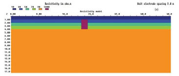
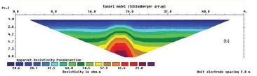
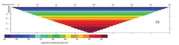
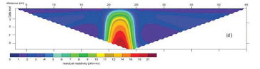
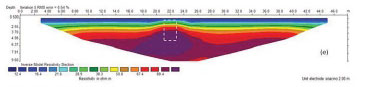
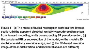
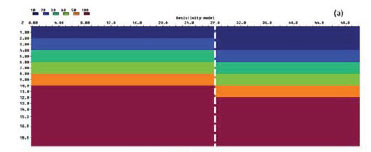
The first model consists of five layers as shown in Figure 1(a). The resistivity values of layers are 10, 30, 50, 70, and 90 Ω-m respectively and the thickness of each layer is considered 1 m. A buried body with dimensions of 2x3 m and a resistivity of 5000 Ω-m is inserted at a burial depth of 1.5 m. The two-dimensional forward model grid has 130*60 nodes. A Wenner-Schlumberger array with 51 electrodes spread at 2 m intervals was modelled. Figures 1(b), 1(c), and 1(d) illustrate the apparent resistivity, BR, and RR pseudo-sections arisen from forward modelling, respectively. Figure 1(e) shows the inversion image from the apparent resistivity data and Figure 1(f) shows the inversion image resulted from the mode's RR data. A comparison between Figure 1(e) and Figure 1(f) shows that the RR-based inversion image illustrates the position and dimensions of the buried body better than the conventional inversion image. It should be noted that as the values are different in the conventional and RR sections (because of subtraction of the BR values from acquired data), the colour scales are chosen such that the anomalies are highlighted in the same pattern.

 

 

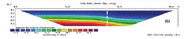
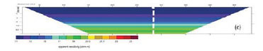
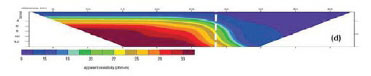
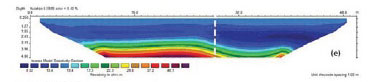
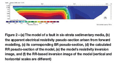
The second model describes a vertical normal fault in a six-strata sedimentary medium. The electrical resistivity values of top layers are 10, 20, 30, 40, and 50 Ω-m respectively, overlying 100 Ω-m bedrock. The thickness of each layer is 2 m (except the covering top layer, which is assumed to be levelled due to erosion), as illustrated in Figure 2(a). The objective of the survey is to detect the position of the fault by using a Wenner electrode array. Figure 2(b) shows the apparent resistivity pseudo-section along the modeled survey line, while Figures 2(c) and 2(d) show its corresponding BR and RR pseudo-sections, respectively. Figure 2(e) shows the conventional inversion image of the model and Figure 2(f) illustrates its RR-based inversion image. As seen in Figure 2(f), the fault location in the RR-based image was determined more accurately than in the conventional image.

 

 

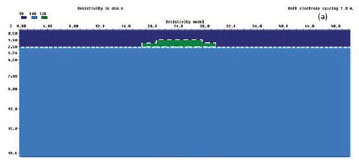
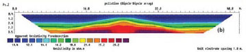
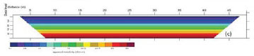
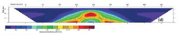
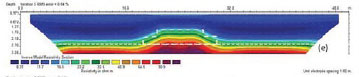
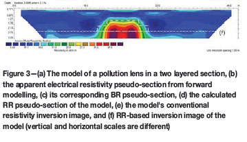
The third model consists of two layers as shown in Figure 3(a). The top layer has an electrical resistivity value of 10 Ω-m and a thickness of 2.5 m. The second layer is a uniform half-space with an electrical resistivity value equal to 100 Ω-m. A horizontal lens with presumed oil pollution and an electrical resistivity value of 120 Ω-m has been inserted in the top layer. The objective is to detect the position and dimensions of the pollution lens by using a dipole-dipole electrode array. Figures 3(b), 3(c), and 3(d) show the apparent resistivity, BR, and RR pseudo-sections along the modelled survey line, respectively. Figure 3(e) shows the model's conventional inversion image and Figure 3(f) illustrates the model's RR inversion image. The comparison between Figure 3(e) and Figure 3(f) shows that the image from the RR inversion yields sharper edges of the pollution lens than the conventional inversion results, although the depth to the top of lens is not well determined.

 

 

Field case study: cavity detection using electrical resistivity method

Zarrinabad karstic limestones are located south of the village of Zarrinabad, 40 km east of Khoram Abad, Lorestan Province, western Iran. Karst caves, usually found in carbonate rocks, can be important geological phenomena near rural and civil regions. In many areas karst aquifers are drinking water resources. Limestone caves exhibit an infinite variety in size and shape (Ford et al., 1988), and may include networks of narrow fissures following the pattern of rock fractures, or rambling mazes of spacious tunnels (Abu-Shariah, 2009). This case study is devoted to an investigation of the existence of probable cavities and their geometry in the Zarrinabad karst area.

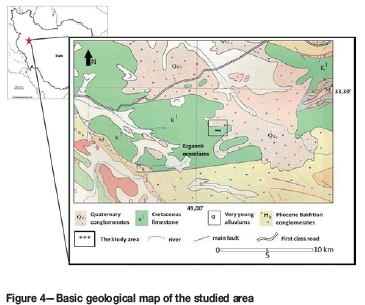
Geologically, the studied area consists of Cretaceous limestone rocks that are partly covered by Quaternary conglomerates. Figure 4 shows a geological map of the studied area. The Cretaceous limestone formation with K^l annotation in the figure extends to the west of the studied area and forms the Ezganeh Mountains. To the east of the study area, Quaternary conglomerates marked with Q^c1 cover the limestone rocks.

 

 

The entrance to a cave that we named Zarrinabad Cave exists at the north side of the studied area. According to the field observations, it is approximately 150 m in length with a nearly north-south trend (Ramazi, 2011).

Survey design

A previous investigation of the area consisted of several vertical electrical soundings using a dipole-dipole electrode configuration. No raw electrical resistivity data is available, except for some hard copies of apparent resistivity contour maps for different array lengths and a report affirming that the applied method could not detect the desired objective(s) properly. According to geological considerations and with regard to geometric and electrical properties of probable cavities in the area, a combined resistivity sounding and profiling electrode array (CRSP) was applied. CRSP was introduced by Ramazi (2005) and is defined as follows: three vertical electrical soundings are surveyed simultaneously by a set of measurement current electrodes that are normally used for one vertical electrical sounding (VES). In this array the distance of each measuring station is equal to the spacing of the potential electrodes (see Figure 5 for a schematic representation of the CRSP array). As shown in the figure, CRSP is similar to the Schlumberger and Wenner-Schlumberger arrays in central measurements; however, the potential electrode spacing can be decreased for shorter current electrode distances and hence increased horizontal resolution obtained. The potential electrode spacing depends on the survey objectives, including the depth of investigation. We define n as:

 

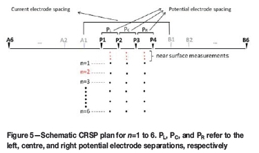
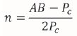
where AB is the current electrode spacing and P_cis the appropriate potential electrode spacing (P₂P₃ distance), which is equal to P_Land P_R. The first current electrode spacing in routine CRSP measurements starts at n=2, which is equal to five times the appropriate potential electrode spacing (including the measuring station interval). For example, if the measuring stations interval is 5 m (P₁P₂ = P₂P₃ = P₃P₄ = 5 m), the first current electrode spacing (AB) for CRSP measurements will be 25 m (AB = 25 m). AB is increased for the other measurements as the following:

For n=1 the current electrode distance is equal to three times the potential electrode spacing (for example AB = 15 m); in this case and also for other near surface measurements (AB<15 m), each the sounding points is surveyed individually as in the Schlumberger array. The data obtained by this array could be processed and interpreted as sounding curves and/or into pseudo-sections. As seen in Figure 5, the CRSP array has the advantage of penetrating deep in the subsurface as well as detecting lateral changes through the acquisition of more data in a section. In practice, CRSP has been successfully applied to different mineral exploration and engineering site investigations (Ramazi and Mostafaie, 2013). It should be noted that a combined method, called 'combined sounding-profiling resistivity' was also proposed by Karous and Pernu (1985). This method is significantly different from CRSP in electrode configuration, field operation, and processing. For example, in the Karous and Pernu proposed array, the distance between potential electrodes is constant, but in the CRSP configuration, three couples of potential electrodes are used (P_L, P_C, and P_R). Likewise, the Karous and Pernu configuration is based on a three-electrode array, while a symmetrical array is used in the CRSP method (Ramazi and Jalali, 2014).

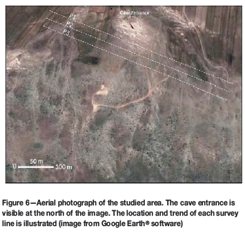
In this case study, CRSP resistivity measurements were acquired along three survey lines. Figure 6 shows the locations of designated survey lines. Each profile was approximately 600 m in length and the distance between two survey lines was set to 30 m. In total, 19 stations (with 57 measurement points) were acquired along each survey line. In all survey lines the measuring point interval as well as potential electrode spacing was assigned as 10 m. Current electrode distances (AB) were selected from 50 m to 250 m. For AB lengths shorter than 50 m, the distance of each couple of the potential electrodes was decreased to 5 m, and each of the sounding points was surveyed separately (n=1).

 

 

 

Results

The RR technique was applied to the acquired data as described above. Figure 7 shows the VES resistivity curve along station 4 of survey line P1. The BR function was calculated using the VES data from station 4 as follows:

 

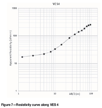
where BR is the background resistivity value of each measuring point and x is the corresponding current electrode spacing (AB).

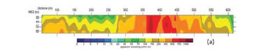
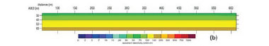
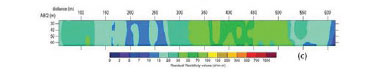
Figure 8(a) illustrates the apparent resistivity pseudo-section along survey line P1, while Figure 8(b) shows its corresponding BR pseudo-section. The RR pseudo-section along survey line P1 is shown in Figure 8(c). Figure 8(d) illustrates the conventional resistivity inversion along survey line P1. As seen from the figure, the formation consists of several resistivity layers that increase in resistivity with depth.

 

 

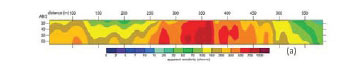
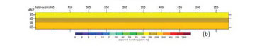
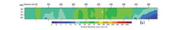
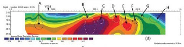
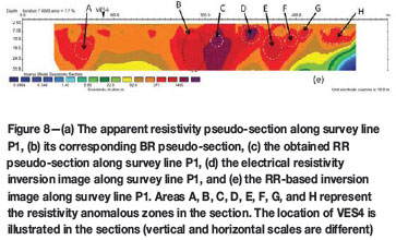
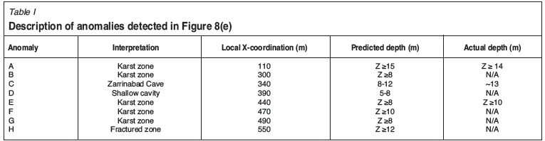
Figure 8(e) shows the RR-based inversion image along P1. The figure shows that by applying the RR method, the rbackground resistivity layers reduce to a relatively more uniform background; moreover, anomalies with high RR values show potential karst cavities (see Table I). The positions of the RR anomalies are also shown in the conventional inversion image in Figure 8(d). According to previous observations, point C represents the Zarrinabad Cave footprint. A comparison between Figure 8(d) and Figure 8(e) clearly shows that the anomalies are considerably more enhanced in the RR-based image. Drill testing into areas A and E convincingly proved the results.

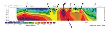
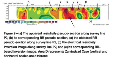
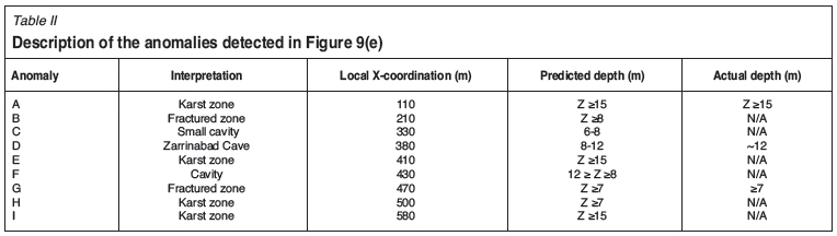
Figure 9(a) shows the apparent resistivity pseudo-section along survey line P2, while Figure 9(b) shows its corresponding BR pseudo-section. The RR pseudo-section along survey line P2 is shown in Figure 9(c). Figure 9(d) represents the electrical resistivity inversion image along survey line P2, while Figure 9(e) shows its corresponding RR-based inversion image. The background resistivity layers in Figure 9(d) were removed in Figure 9(e). Area D in the figure shows the footprint of Zarrinabad Cave. Areas A and H in Figure 9(e) represent RR anomalous zones that were concealed by the natural regional resistivity gradient in Figure 9(d). Table II describes anomalies detected in the figure.

 

 

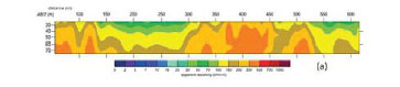
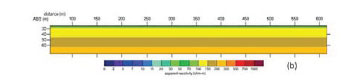
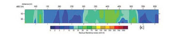
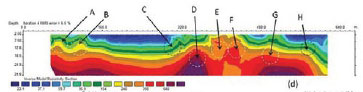
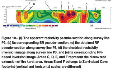
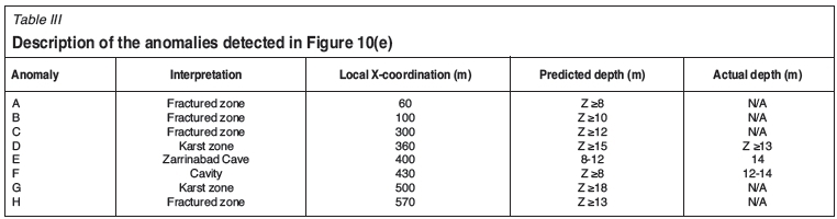
The apparent resistivity pseudo-section along survey line P3 is shown in Figure 1(a), while Figure 10(b) shows its corresponding BR pseudo-section. Figure 10(c) also illustrates the RR pseudo-section along survey line P3. Figure 10(d) shows the electrical resistivity inversion image along survey line P3, and Figure 10(e) represents its corresponding RR-based inversion image. A visual comparison of Figure 10(d) and Figure 10(e) highlights the proficiency of the RR technique well. The RR anomalous zones of areas C, D, E, and F in Figure 10(e) completely distinguish shallow karst zones, their extensions, and probable connections. Further drilling into area D proved this interpretation. Areas E and F in Figure 10(e) represent Zarrinabad Cave footprints. Areas A, B, C, G, and H in Figure 10(e) represent several anomalous RR zones, which are faded in the conventional electrical resistivity inversion image (Figure 10(d)), suggesting filled or small cavities. This interpretation has not been drill-tested (Table III).

 

 

Conclusions

In this paper the residual resistivity (RR) technique was introduced as a new method of electrical resistivity data processing. The RR technique can enhance probable local anomalies through the elimination of regional resistivity gradients. The technique may highlight positive and/or negative anomalies representing materials with electrical resistivity values more or less than the background level respectively. The most important conclusions are summarized as follows:

> Background resistivity plays an important role in resistivity anomaly detection. In many cases it changes due to variations in physical properties of the investigated area (as in the synthetic and field case studies)

> The existence of potentially fictitious anomalies is reduced by the RR technique due to the determination of the background resistivity gradient for each measuring point. Likewise, probable anomalies that are not easily detectable by conventional inversion methods are highlighted with acceptable precision and resolution

> Shallow and deep underground cavities were detected in the Zarrinabad karst area by applying the RR technique. Further drilling convincingly proved the results obtained by this technique

> The CRSP (combined resistivity sounding and profiling) electrode array is an appropriate array for applying the RR technique.

 

References

Abu-Shariah Mohamad, I.I. 2009. Determination of cave geometry by using a geoelectrical resistivity inverse model. Engineering Geology, vol. 105. pp. 239-244.         [ Links ]

Aizebeokhai, A.P., Olayinka, A.I., and Singh, V.S. 2010. Application of 2D and 3D geoelectrical resistivity imaging for engineering site investigation in a crystalline basement terrain, southern Nigeria. Environmental Earth Sciences, vol. 61. pp. 1481-1492.         [ Links ]

Bayrak, M. and Senel, L. 2012. Two-dimensional resistivity imaging in the Kestelek boron area by VLF and DC resistivity methods. Applied Geophysics, vol. 82. pp. 1-10.         [ Links ]

Candansayar, M.E. and Basokur, A.T. 2001. Detecting small scale targets by the 2D inversion of two-sided three-electrode data: application to an archeological survey. Geophysical Prospecting, vol. 49, no. 1. pp. 13-25.         [ Links ]

De La Vega, M., Osella, A., and Lascano, E. 2003. Joint inversion of Wenner and dipole-dipole data to study gasoline-contaminated soil. Applied Geophysics, vol. 54. pp. 97-109.         [ Links ]

Fehdi, C., Baali, F., Boubaya, D., and Rouabhia, A. 2011. Detection of sinkholes using 2D electrical resistivity imaging in the Cheria Basin (north-east of Algeria). Arabian Journal of Geosciences, vol. 14, no. 1-2. pp. 181-187.         [ Links ]

Ford, D.C., Palmer, A.N., and White, W.B. 1988. Landform developments; karst. The Geology of North America. Vol. O-2, Hydrogeology. pp. 401-412.         [ Links ]

Ha, H.S., Kim, D.S., and Park, I.J. 2010. Application of electrical resistivity techniques to detect weakand fracture zones during underground construction. Environmental Earth Sciences, vol. 60. pp. 723-731.         [ Links ]

Loke, M. 1995-2013. RES2DMOD, 2D resistivity and IP forward modeling, Ver. 3.0. www.geotomosoft.com/r2dmodwin.zip [Accessed 12 June 2014].         [ Links ]

Loke, M. and Barker, R. 1996. Rapid least squares inversion of apparent resistivity pseudo-sections using a quasi Newton's method. Geophysical Prospecting, vol. 44. pp. 131-152.         [ Links ]

Kamkar-Rouhani, A. 1998. Development and application of processing techniques for signal enhancement using multisystem resistivity measurements. PhD thesis, Curtin University of Technology, Australia.         [ Links ]

Karous, M. and Pernu, T.K. 1985. Combined sounding-profiling resistivity measurements with the three-electrode arrays. Geophysical Prospecting, vol. 33. pp. 447-459.         [ Links ]

Niwas, S.M. and Mehrotra, A.M. 1997. A stable iterative scheme for inversion of direct current resistivity sounding data. Acta Geodaetica et Geophysica Hungarica, vol. 32, no. 1-2. pp. 15-25.         [ Links ]

Nordiana, M.M., Rosli, S., and Nawawi, N.N.M. 2014. A numerical comparison of enhancing horizontal resolution (EHR) technique utilizing 2D resistivity imaging. Arabian Journal of Geosciences, vol. 17, no.1. pp. 299-309.         [ Links ]

Oldenburg, D.W. and Lí, Y. 1994. Inversion of induced polarization data. Geophysics, vol. 59. pp. 1327-1341.         [ Links ]

Papadopoulos, N.G., Tsokas, G.N., Dabas, M., Yi, M. and Tsourlos, P. 2009. 3D inversion of Automated Resistivity Profiling (ARP) data. ArcheoSciences, vol. 33 (suppl.). pp. 329-332.         [ Links ]

Ramazi, H.R. 2005. Combined resistivity sounding and profiling and its application in mineral exploration and site investigation. Technical report. Zamin Moj Gostar, Tehran, Iran. 21 pp. (in Persian).         [ Links ]

Ramazi, H.R. 2011. Zarrinabad karsts geophysical report. Zamin Moj Gostar, Tehran, Iran. 100 pp. (in Persian).         [ Links ]

Ramazi, H.R. and Jalali, M. 2014. Contribution of geophysical inversion theory and geostatistical simulation to determine geoelectrical anomalies. Studia Geophysica et Geodaetica, vol. 59, no. 1. pp. 97-112. DOI: 10.1007/s11200-013-0772-3        [ Links ]

Ramazi, H.R. and Mostafaie, K. 2013. Application of integrated geoelectrical methods in Marand (Iran) manganese deposit exploration. Arabian Journal of Geosciences, vol. 6, no. 8. pp. 2961-2970.         [ Links ]

Smith, N.C. and Vozzof, K. 1984. Two dimensional DC resistivity inversion for dipole- dipole data. IEEE Transactions on Geosciences and Remote Sensing, vol. GE-22, no. 1. pp. 21-28.         [ Links ]

Wilkinson, P. B., Meldrumm, P.I., Kuras, O., Chambers, J.E., Holyoake, S.J., and Ogilvy, R.D. 2010. High-resolution electrical resistivity tomography monitoring of a tracer test in a confined aquifer. Applied Geophysics, vol. 70. pp. 268-276.         [ Links ]

Yilmaz, S. and Narman, C. 2014. 2-D electrical resistivity imaging for investigating an active landslide along a ridgeway in Burdur region, southern Turkey. Arabian Journal of Geosciences. DOI: 10.1007/s12517-014-1412-0.         [ Links ]