PAPERS - CHEMICAL ENGINEERING & METALLURGY AT WITS

 

Optimization of complex integrated water and membrane network systems

 

 

M. Abass; E. Buabeng-Baidoo; D Nezungai; N. Mafukidze; T. Majozi

School of Chemical and Metallurgical Engineering, University of Witwatersrand, Johannesburg

 

 

---

SYNOPSIS

Water and energy are key resources in the process and mining industries. Increasing environmental and social pressures have made it necessary to develop processes that minimize the consumption of both these resources. This work considers the synthesis and optimization of water networks through partial treatment of water (regeneration) before recycle/re-use. Two types of membrane regenerators are considered, namely electro-dialysis and reverse osmosis. For each of the membrane regenerators, a detailed design model is developed and incorporated into the water network model in order to minimize water and energy consumption, and operating and capital costs. This represents a rigorous design and accurate cost representation as compared to the 'black-box' approach. The presence of continuous and integer variables, as well as nonlinear constraints, renders the problem a mixed integer nonlinear programming (MINLP) problem. Four cases are presented. The first case looks at the incorporation of multiple electrodialysis regenerators with single contaminant streams within a water network (WN), while the second considers the multiple contaminant scenario. Case 3 examines the incorporation of a reverse osmosis network superstructure within a WN, and case 4 looks at both electrodialysis and reverse osmosis membranes. The developed models are applied to a pulp and paper and a petroleum case study to demonstrate their applicability, assuming both a single and multiple contaminant scenario. The model was solved in GAMS using BARON and DICOPT. The results indicate a wastewater reduction of up to 80% and savings of up to 44% in fresh water intake, 82% in energy, and 45% in the total annualized cost.

Keywords: sustainable, synthesis, optimization, reverse osmosis, electrodialysis.

---

 

 

Introduction

Water and energy are important resources for the development and wellbeing of humanity. They are key components in both the process and the mining industry, and great amounts of each resource are consumed to produce the other. Process integration is often employed in order to establish a holistic water network superstructure for minimizing the consumption of water and energy. This is done through an integrated water network that is open for direct re-use, recycle, and regeneration re-use/recycle for sustainable, cost-effective water and energy usage.

Water pinch techniques and mathematical-based optimization techniques are the two main approaches used for optimal synthesis of water networks in the process industries. Wang and Smith (1994, a, b) presented the seminal work in water pinch analysis which sets to target the re-use, regeneration, and reuse/recycle of waste water in order to reduce fresh water consumption. That work has since developed into advanced graphical, tabular, and heuristic methods for water network synthesis. The insight-based techniques do not involve computational algorithms in generating solutions. They do, however, require significant problem simplifications and assumptions, and are inherently limited to mass-transfer-based operations (Manan et al., 2004; Bandyopadyay and Cormos, 2008; Tan et al., 2009).

Takama et al. (1980) presented a superstructure optimization approach for water minimization in a petrochemical refinery based on a fixed mass load. The work was later extended by several other researchers (Rossiter and Nath, 1995; Doyle and Smith, 1997; Huang et al., 1999; Karrupiah and Grossmann, 2006; Ahmetovic and Grossmann, 2010). Quesada and Grossmann (1995), Karrupiah and Grossmann (2006), and Faria and Bagajewicz (2011) presented algorithms to obtain feasible solution in cases of the more complex nonlinear programming (NLP) and mixed integer nonlinear programming (MINLP) problems that are in many cases a challenge to solve. Mathematical optimization allows water network synthesis problems to be treated in their full complexity by considering representative cost functions, multiple contaminants, and various topological constraints (Takama, et al., 1980; Savelski and Bagajewicz, 2000; Bagajewicz and Savelski, 2001; Grossman and Lee, 2003; Gunaratman et al., 2005). Mathematical optimization approaches also have an added advantage of simulating the water network into a desired network structure and operational condition (Chew et al., 2008).

Tan et al. (2009) presented a water network superstructure with a single membrane partitioning regenerator which allows for possible re-use/recycle. The work considered the 'black-box' approach, which uses linear cost functions for the membrane regenerators. This does not give an accurate cost representation of the water network. Khor et al. (2011) addressed this deficiency by developing a detailed model representation for water network regeneration synthesis using a MINLP optimization framework. This work of was, however, limited to a single regenerator with a fixed design. In a more recent development, Yang et al. (2014) proposed a unifying approach by combining multiple water treatment technologies capable of treating all major contaminants. The work focused on unit-specific short-cut cost functions in order to gain detailed understanding of tradeoffs between efficiency of treatment units and the cost of the units, as well as the impact on the unit design. To date, all the work on water and membrane regeneration has focused on minimizing water usage and the cost functions of the water networks. No effort has been devoted to the simultaneous synthesis of the membrane regeneration units and water network for water and energy minimization.

The membrane technologies adopted in the current work are electrodialysis (ED) and reverse osmosis (RO). Electrodialysis is based on the electromigration of ions through cation and anion exchange permselective membranes by means of an electrical current (Korngold, 1982; Tsiakis and Papageorgiou, 2005; Strathmann, 2010). Industrial applications of ED include brackish water desalination, boiler feed and process water, and wastewater treatment (Strathmann, 2010). The current work employs insights on the mathematical relations in the work of Lee et al. (2002) and Tsiakis and Papageorgiou (2005).

RO is a pressure-driven membrane separation process that selectively allows the passage of one or more species through the membrane unit. Industrial applications of RO include municipal and industrial water and wastewater treatment. It has also gained widespread industrial usage in partitioning regenerators to enhance water quality for reuse/recycle (Garud et al., 2011). A detailed mathematical model of an RO unit that allows for process simulation and optimization has been developed by El-Halwagi (1997).

In the application of membrane systems as regenerators in water network optimization for wastewater reduction, an enormous amount of energy is used. Most published work, however, uses linear cost functions and 'black-box' representation for membrane partitioning regenerators (Alva-Argáez et al., 1998; Tan et al., 2009; Khor et al., 2012). This does not result in an accurate cost representation of the membrane systems. There is thus an opportunity for energy minimization through detailed synthesis of membrane regeneration systems in order to obtain optimal variables that affect the operation and economics of the regenerator unit.

The main objective of the current work is to develop an integrated water and membrane regeneration network superstructure that incorporates possibilities for water and energy minimization. The membrane regenerators in this representation are ED and RO. The choice of regenerators is motivated by the increasing use of membrane technology for water treatment in the process and mining industries, and also the potential of different membrane systems to treat specific ranges of waste. A detailed synthesis of the membrane regeneration systems is conducted to determine optimal operating conditions for efficient energy usage in terms of costs. The detailed model of the regenerators is incorporated in the overall water network objective function in order to minimize fresh water and energy consumption, and also give a true representation of costs as compared to the 'black-box' method. The idea of using variable removal ratios to describe the performance of regenerators is also explored.

 

Problem statement

The main aim of this study is to develop a water network superstructure for the synthesis of a combined water and membrane network for water and energy minimization based on the following data:

> A set of water sources, J, with known flow rates and contaminant concentrations

> A set of water sinks, I, with known flow rates and known maximum allowable contaminant concentrations

> A set of membrane regeneration units, R, with the potential for parallel/series connection for partial treatment of wastewater from sources for re-use/recycle

> A fresh water source, FW, with known concentration, and variable and unlimited flow rate

> A wastewater sink, WW, with maximum allowable contaminant concentration, and variable and unlimited flow rate.

The following outputs are required:

> The minimum fresh water intake and wastewater generation, the energy consumed in the ED and RO units, and the total annualized costs for ED (TAC_e) and RO (TAC_r)

> Optimal water network configuration

> Optimum design variables of the regenerators.

 

Superstructure representation

Based on the problem statement, the water network superstructure in Figure 1 is developed. The superstructure representation is an extension of the work by Khor et al. (2011). The superstructure in this work incorporates multiple regenerators which are open for parallel and series connection as well as recycle and re-use of both permeate and reject streams from the regenerators. The fixed flow rate approach adopted in this work considers water-using processes in terms of sources and sinks that generate or consume a fixed amount of water respectively. Total fixed flow rate is adopted because it presents a general representation of water-using operations based on both mass transfer and non-mass transfer (Khor et al., 2012).

 

Model development and application

This work considers four different cases, all of which are based on the superstructure given in Figure 1.

> Single contaminant, multiple ED units

> Multiple contaminants, single ED unit

> Multiple contaminants, multiple RO units

> Single contaminant, ED and RO units

For each of the cases considered the model is applied to a case study. For comparison, different modelling scenarios are presented for each case.

Case 1: single contaminant and multiple ED units

This case considers the synthesis of an optimal water network with multiple ED regenerators using a single contaminant framework. The model is made up of water balances of the entire network and the mechanistic model of the regeneration network. The detailed model of the regeneration subnetwork incorporated in the network allows for the design of the subsystem.

Mathematical model water balances

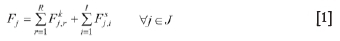
To ensure connectivity between the regeneration network, the sources, and the sinks, water balances are established based on the superstructure presented in Figure 1. The flow balance for the source is modelled as:

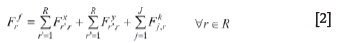
The balance for the fresh water source is modelled in a similar way. Material balances on the regeneration network show the connectivity between individual regenerators and the rest of the water network. The water balance around the mixer preceding each regenerator can be modelled as:

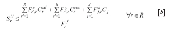
Depending on the design of the regenerator, each regenerator has a limit to the amount of contaminant that it

can tolerate. In this regard, the corresponding contaminant balance for the regenerator feed was modelled as:

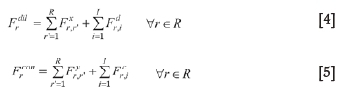
Similarly, the water balances for the two splitters connected to the regenerator diluate and concentrate streams are given by the constraints in Equations [4] and [5] respectively.

The flow balance for the sink is modelled as:

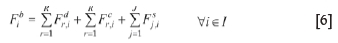
The balance for the wastewater sink is modelled in a similar way. The maximum allowable load that each sink tolerates has to be taken into account. As such, the corresponding contaminant balance for each sink can be modelled as:

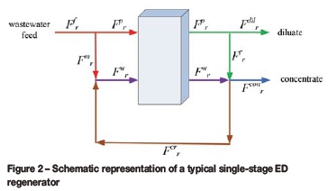
Mechanistic ED regeneration network model

The model formulation for the detailed design of the ED regeneration unit is based on the work by Tsiakis and Papageorgiou (1995) and Lee et al. (2002). Figure 2 is a schematic representation of a typical ED unit. For computational simplicity, one stage per regenerator is assumed.

 

 

The following assumptions are made in order to describe the plant using a set of mathematical equations describing its operation.

> The fluids considered are Newtonian and have steady, fully developed, incompressible laminar flow

> The unit is operated under a co-current set-up

> Concentrate and diluate cells have identical geometry and flow patterns and changes in the ohmic resistance of the solutions are negligible (Tsiakis and Papageorgiou, 1995)

> The concentrations of the salt species are operated using molar equivalents

> Water transportation across the membrane is negligible compared to the concentrate and diluate stream flow rates (Tsiakis and Papageorgiou, 1995)

> To avoid the collapse of the membrane system due to pressure differences it is assumed that the immediate diluate and concentrate streams have the same flow rate.

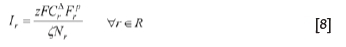
Water balances as well as corresponding contaminant balances for each regenerator were conducted in accordance with Figure 2. With regard to the design aspect of ED regenerator, important variables and physical parameters of the ED are incorporated in the mathematical relations that describe the performance of the regenerator. The electrical current required to drive the ED process is given by:

The extent of desalination obtained by an ED unit is dependent on the membrane area, A_r, which based on Tsiakis and Papageorgiou (1995), and given by:

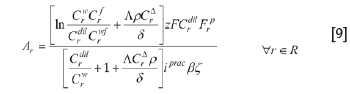
where, C_ris the concentration difference across a stage (C^f_r - C^dil_r). F^p_ris the diluate stream flow rate from the regenerator, r, which is expressed by Equation [10].

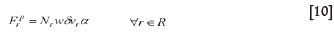
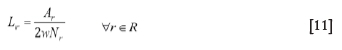
where a is the spacer shadow factor. The required process path length for the ED stack can be expressed in terms of the membrane area, A_r, the cell width, w, and the number of cell pairs, N_r, as follows:

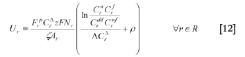
The direct energy required for the process is dependent upon the voltage and current applied on each stack. The voltage applied can be expressed as follows:

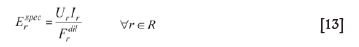
The specific energy required for desalination is defined by:

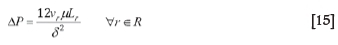
The specific pumping energy, E_r^pump, required for the process is directly linked to the pressure drop, ΔP_r, for laminar flow across the unit and is given by:

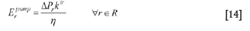
where

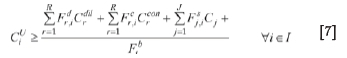
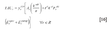
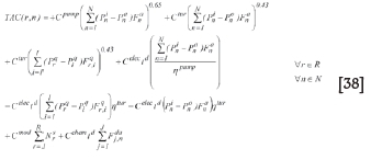
The regeneration subnetwork involves both capital and operational costs. The representative total annualized cost (TAC) function for the regeneration network is given by Equation [16]. This function is included in the overall objective function of the water network, such that the energy consumption and subsequent cost of regeneration are minimized in conjunction with water consumption. The model is enabled to select only the necessary regenerators that result in an optimal solution by prefixing the TAC function with a binary variable, y_r^ED, which becomes zero when the respective unit is not activated.

The objective function

The objective is to minimize the total annualized cost of the water network, which comprises the fresh water cost, wastewater treatment cost, annualized regeneration cost, as well as the capital and operating cost of piping. The formulation of the objective function is expressed in Equation [17].

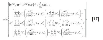
where

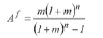
is an annualization factor. It is assumed that all the pipes share the same p and q parameter properties, stream velocity v, and 1-norm Manhattan distance. The resulting mathematical model is a MINLP problem that was solved using GAMS/DICOPT with CPLEX as the MILP solver and CONOPT 3 as the NLP solver. BARON was used to solve the RMINLP problem.

Illustrative example

The mathematical model developed is applied to a literature-based pulp and paper plant case study (Chew et al., 2008). The industry produces a lot of ionic effluent and also involves miscible water networks, whereby the mixing streams lose their identities as they mix. This renders the fixed flow rate framework adopted in the model ideal for this particular plant (Poplewski et al., 2010). The limiting data is shown in Table I.

Three scenarios are considered. Scenario 1.1 is water integration without regeneration. Scenario 1.2 considers a water network with one detailed ED regenerator with capabilities of recycle within the regeneration subnetwork.

Note that within this scenario two cases were considered; that is, the case where the removal ratio of the regenerator is fixed at 0.733 and the case where it is variable. For the case where the removal ratio is fixed, an arbitrary value is chosen. Scenario 1.3 is similar to scenario 1.2 except that it has the capability of using two regenerators. Fixed removal ratios of 0.733 and 0.950 for the first and second regenerators, respectively, are chosen for the fixed removal ratio case.

Comparisons of the presented cases show that Scenario 1.3 is the most preferable, since the largest amount of water was treated at the lowest total cost, thereby minimizing the fresh water intake and wastewater generation. It is evident from Table II that by allowing the solver to choose the optimal configuration within the regeneration subnetwork in terms of recycles, series and parallel connections, as well as making the removal ratio and number of regenerators required variable, there is the possibility of obtaining better solutions rather than fixing them arbitrarily beforehand. In this way the designer gains more control of the unit performance by being able to stipulate the required membrane characteristics to the manufacturer.

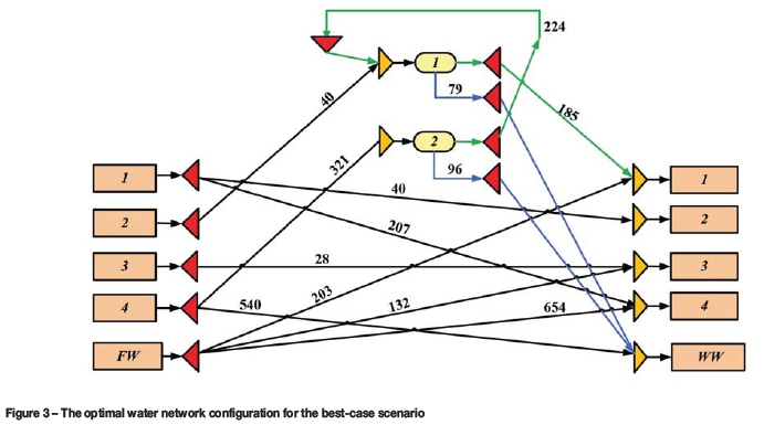
The results also show that incorporating multiple regenerators can increase the chances of a better optimal solution, as long as the regenerators are not forced into the system. In this case this situation was handled by the binary variable y_r^EDthat represented the existence of a regenerator which allowed the optimization tool to decide on the optimum number of regenerators. Figure 3 shows the optimal network configuration and flow rates for the best-case scenario. All flowrates are reported in kg/s.

With this configuration in place, the plant is capable of generating savings of up to 12.7% in fresh water intake, reduction of up to 16.2% in wastewater generation, and a 14.1% saving in the total annualized cost compared to the worst-case scenario. The optimal regenerator design suggests an installation of two regenerators, r₁and r₂, one with 2880 cell pairs and the other with 4356, amounting to a total membrane area of 3837 m² and 3921 m² respectively. It is noteworthy that the CPU time incurred was high for scenario 1.3, due to the nature and complexity of the model.

Case 2: multiple contaminants and single ED unit

In this case, it is necessary to develop a multicontaminant model for ED design. This requires the consideration of the ionic interaction between the different components within the ED unit, and the impact of these interactions on the unit design. In the following formulation, the subscript r is omitted from the notation because only a single regenerator is considered.

Mathematical model

The individual concentrations of the contaminants feeding into the ED unit are combined using an equivalent concentration expression, as defined in Equation [18],where subscripts c, a, and s denote the cation, anion, and salt respectively. All calculations pertaining to the ED unit were performed using an equivalent concentration. However, the subscript eq has been omitted for clarity.

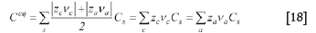
The calculation of equivalent concentration must be performed in all streams entering and exiting the ED unit as follows:

The solution conductivity is a fundamental property of the fluid that plays an integral part in determining the ED design. It must, therefore, be determined based on the actual concentration of the contaminants that enter the unit. This can be done empirically or analytically by the use of conductivity-concentration relationships such as the Deybe-Huckel-Onsager. The latter approach is adopted in this work. It is important to note that as the complexity of the electrolytes increases, such relationships become less accurate, and experimental determination of the dependence of solution conductivity on salt concentration is advised. The Deybe-Hückel-Onsager equation is given by Equation [22]:

 

In this expression, a refers to the fraction of the salt in the solution and k is the specific conductance of the solution or the individual components. In order to relate the specific conductance to the solution conductivity, the following relationship is employed

This expression can be applied to both the individual electrolytes and the overall solution. The combination of these three equations allows one to calculate the conductivity of a solution given the individual concentrations and their infinite conductivities.

Electrical current

The following ED energy minimization model was developed for a single-stage process. The electrical current is determined using a modified form of Faraday's law. This expression relates the driving force with the physical characteristics of the plant, the required capacity and the degree of desalination. Either the cationic or anionic valence and stoichiometric coefficients may be used in Equation [25].

The practically applied limiting current density, beyond which the ED must not operate, is given by the empirically determined relationship:

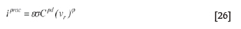
Coefficients σ and φ are experimentally determined constants, u is the fluid velocity, and e is a practicality factor that relates the limiting current density to the unit's flow patterns.

Design considerations

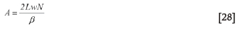
While many of the design constraints are similar to the single contaminant case as described above, some modifications must be made to incorporate the equivalent concentrations for the multicontaminant case. The total length of the ED stack is given by the following relationship:

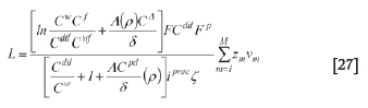
The conductivity, Λ, is determined using the constraints in Equations [22]-[24]. The corresponding required membrane area is determined as a function of the path length and the cell width. A correction factor, β, is introduced to account for the effect of the spacers.

Energy considerations

The energy consumption in an ED unit can be attributed to the migration of electrons across the membranes as well as the energy required to pump fluids through the unit. Assuming that operation is ohmic, i.e. current density does not exceed limiting current density, the voltage across the unit is given by:

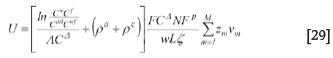
The specific energy for desalination and pumping energy are subsequently calculated using Equations [13] and [14].

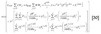
Objective function

The water network and ED model culminate in an overall cost function to be minimized, given by Equation [30]. All pipes are assumed to operate at the same fluid velocity, U_p, and use the same costing coefficients p and q. The piping cost is calculated as a function of the Manhattan distance, D, between any two units.

Illustrative example

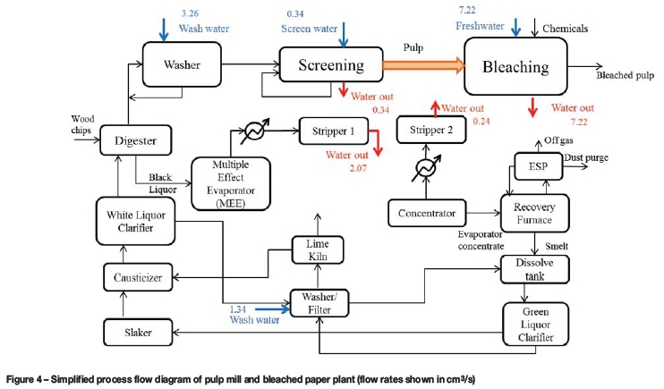
The above model is applied to a pulp mill and bleached paper plant adapted from Chew et al. (2008). In the original scenario, shown in Figure 4, four separate fresh water feeds are used, with a total consumption of 8500 t/d, and four separate effluent streams are produced, totalling 10 500 t/d.

Two contaminants were identified, namely NaCl and MgCl2. The flow rates and contaminant concentrations of the sources and sinks are detailed in Table III. Two process integration scenarios were compared. In both cases, the model was solved using GAMS/BARON.

> Scenario 2.1: a 'black-box' model is used and the costing of the actual required ED unit is performed separately, i.e. water minimization only

> Scenario 2.2: simultaneous minimization of water and energy, using the developed model. Input data for the ED units was kept constant for comparison between the two scenarios.

Water minimization

In this scenario, the objective is water minimization. The water regeneration is represented only by a constant removal ratio and a linear cost expression. The actual ED cost is determined based solely on the throughput. The results from the WNS are then input to a standalone ED model in order to determine the true cost of regeneration under these conditions.

A full range of results is given in Table IV. Simple water minimization results in a 36% saving in fresh water and 60% reduction in wastewater generated, compared to the original plant. A comparison between the estimated and true costs of regeneration highlights the inaccuracies involved when a linear cost function is applied to a nonlinear membrane process. The linear cost function considers only the flow rate of feed to the ED; the true cost is determined by all aspects of the units design. Table IV shows that there is an 85% discrepancy between the 'black-box' estimate of regeneration cost and the cost of the actual required ED unit under the same conditions. The 'black-box' approach presents the risk of misrepresenting the water network, resulting in suboptimal solutions.

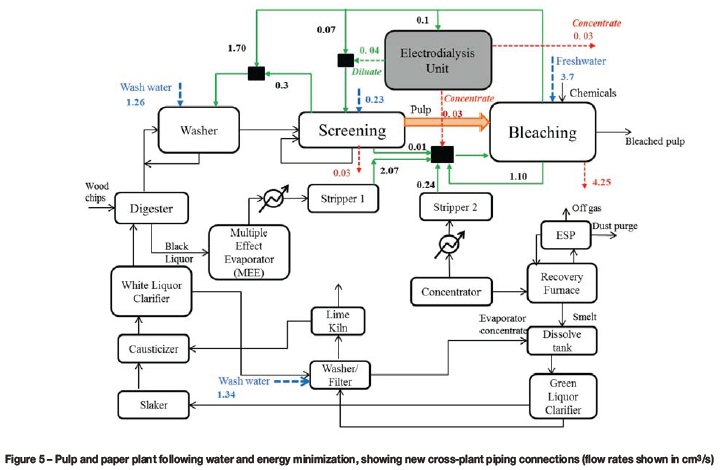
Water and energy minimization

In the water and energy minimization case, the entire model, including the detailed ED, was used, with the same inputs as in the first scenario. The final plant configuration is shown in Figure 5.

A comparison between the ED units from scenarios 1 and 2 shows that when the optimization of the ED is embedded into the water network the required unit has a more conservative design and therefore consumes less energy. Table V shows key variables determined in the optimization, highlighting the comparison between the two scenarios. The integrated approach, therefore, results in an 80% reduction in the overall cost of the ED unit required.

 

 

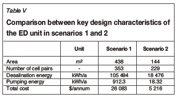
Key characteristics of the models are presented and compared in Table V. While the model sizes are similar, the time taken to solve the integrated model (scenario 2) was close to 21 hours, while the 'black-box' (scenario 1) required only 2 minutes. This can be attributed to the nonlinearity of the ED model combined with the already nonconvex WNS model. It is necessary, therefore, to further develop the model to reduce its computational complexity, which will constitute future work.

Case 3: multiple contaminants, multiple RO units

This case work proposes a superstructure optimization for the synthesis of a detailed RON within a WNS. A rigorous nonlinear RON superstructure model, which is based on the state space approach by El-Halwagi (1992), is included in the WNS to determine the optimum number of RO units, pumps, and turbines required for an optimal WNS. A fixed flow rate model that considers the concept of sources and sinks is adopted. The model takes into account streams with multiple contaminants. The idea of using a variable removal ratio to describe the performance of the regenerators is also explored in this case. The water balances are similar to those proposed in case 1.

Mathematical model

Reverse osmosis constraints

The characteristics of the RO membrane need to be described in order to relate flow rate to pressure. The pressure drop across the membrane ΔP_ris given in Equation [31] (Khor et al., 2011). The equation was simplified by assuming a linear-shell side concentration and pressure profiles (El-Halwagi, 1997).

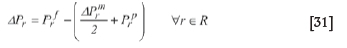
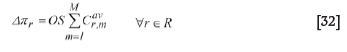
The osmotic pressure, Δπ_r, is defined as a function of the contaminant concentration on the feed side (Saif, Elkamel, and Pritzker, 2008a) and is shown in Equation [32].

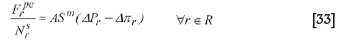
The permeate flow rate per module is given in Equation [33].

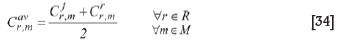
The average concentration C_q^av_mon the feed side is given by Equation [34].

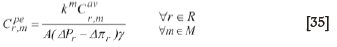
The concentration of contaminants on the feed side must also be described in terms of the pressure drop and the osmotic pressure. This is described in Equation [35].

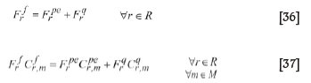
A mass and concentration balance around the regenerator is also needed and is described in Equations [36] and [37] respectively.

Objective function

The objective function of the combined RON superstructure and WNS is used to minimize the overall cost of the regeneration network on an annualized basis which consists of:

> TAC of the RON

> Cost of fresh water (FW)

> Treatment cost of wastewater (WW) > Capital and operation costs of the piping interconnection.

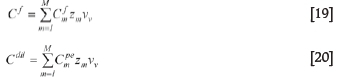
The total annualized cost of the RON consists of the capital cost of the RO modules, pumps, and energy recovery turbines, operating cost of pumps and turbines, as well as pretreatment of chemicals. The operating revenue of the energy recovery turbine is also considered in the determination of the TAC and is shown in Equation [38]. The set n represents the mixing node before a regenerator unit and is used to connect the water network to the RON superstructure.

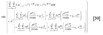
The piping cost of components is formulated by assuming a linear fixed-charge model. In the formulation, a particular cost of a pipe is incurred if the particular flow rate through the pipe falls below the threshold value. This is achieved by using 0-1 variables. Equation [39] represents the objective function of the total regeneration network.

The overall model results in a nonconvex MINLP due to the bilinear terms as well as the power function in the constraints.

Illustrative example

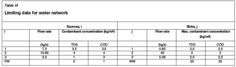
The above model was applied to a petroleum refinery case study based on the work presented by Khor et al. (2011). The model was implemented in GAMS 24.2 using the general purpose global optimization solver BARON, which obtains a solution by using a branch-and-reduce algorithm. The network consists of four sources and four sinks. The limiting water data for the sources and sinks is given in Table VI.

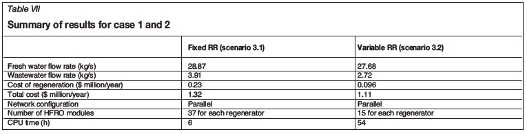
Table VII shows the comparison between a case where multiple regenerators with fixed (scenario 3.1) and variable removal ratio (scenario 3.2) were used. The removal ratio chosen by the model in scenario 3.2 was 0.97 for all contaminants instead the fixed value of 0.95 in scenario 3.1. Scenario 3.2 led to 3.12% reduction in fresh water and 30.43% reduction in wastewater generation in comparison with scenario 3.1. A 15.91% reduction in the total network cost was also achieved. The large decrease in the total cost of the network in scenario 3.2 can be attributed to the higher removal ratio selected by the model than the value that was initially predicted. The modelling of scenario 3.2 is, however, computationally expensive as can be seen in Table VII.

Figure 6 shows the water network for scenario 3.2 with the corresponding flow rate for each stream. The best case used 15 HFRO modules per regenerator. The model selected two regenerators, two pumps, and two energy recovery turbines, as can be seen in Figure 6. It can also be seen that a parallel configuration of the network was chosen by the model. In comparison with the case where no regeneration was considered, scenario 3.2 leads to a 28% reduction in fresh water consumption and 80% reduction in wastewater generation.

 

The long computational time for solving the model in scenario 3.2 was due to the complexity of the problem as well as the large number of 0-1 variables. The model solves quicker when tighter bounds are imposed on the feed and retentate pressure. The use of the energy recovery turbines in the RON led to a reduction in the regeneration cost of the network, and as a result, a reduction in energy usage by the system was achieved.

Case 4: single contaminant, multiple RO and ED units

In this case, an integrated water network of ED and RO unit is developed with the possibilities of water and energy minimization. The choice of regenerators is motivated by the increasing demand for and use of membrane technology for water treatment and also the varying potential of different membrane systems to treat specific waste ranges.

Mathematical model

The model formulation in this representation included constraints for mass and concentration balances of the ED and RO units in cases 1 and 2, detailed formulation of the ED and RO unit respectively, and the overall total annualized costs of both regeneration units represented in cases 1 and 2, which is incorporated in the objective function as follows.

Objective function

Equation [40] represents the objective function that minimizes the overall annualized cost of the water network. This includes fresh water cost, wastewater treatment cost, and annualized regeneration cost, as well as capital and operating costs of piping interconnections. The costs related to piping are accounted for by specifying an approximate length of pipe, the material of construction, and linear velocities through the pipes.

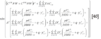
A 1-norm Manhattan distance is considered for all piping interconnections. All pipes are assumed to be of the same material of construction; as a result, the carbon steel pipe parameters of p and q are adopted for the piping costs. Af is the annualization factor adopted from Chew et al. (2008) which is used to annualize the piping cost. The resulting mathematical model is a MINLP. The nonlinear terms are due to the presence of bilinear terms in mass balance equations and power terms in the cost functions of regeneration units. The MINLP model was solved using GAMS 24.2, using the general-purpose global optimization solver BARON.

Illustrative example

The developed mathematical model is verified and applied to the pulp and paper case study adopted from Chew et al. (2008). The choice of the case study is motivated by the high amount of ionic components produce by the pulp and paper industry. Moreover, the pulp and paper industry involves miscible phase networks that consist of water-water systems where streams lose their identities through the mixing process, hence the case study is suitable for a fixed flow rate method adopted for this work.

Table VIII shows the basic data for the plant water network, which comprises five water sources, including the fresh water source, and five water sinks, including the waste sink.

The case study was applied to three different model cases in order to ascertain the benefits of incorporating a detailed network of the membrane regeneration units in the constraints of the water network.

> Scenario 4.1 considered a model of the water network without regeneration

> Scenario 4.2 considered a model of water network with regeneration units based on the 'black-box' approach

> Scenario 4.3 considered a detailed synthesis of the regeneration units incorporated into the overall water network objective function.

For scenarios 4.2 and 4.3, the optimization was conducted for both a fixed and a variable removal ratio. For comparison, in both scenarios the removal ratio had a fixed value of 0.7.

The optimal results for all scenarios are presented in Table IX. Scenario 4.1 represents the water network model without regeneration. Scenario 4.2 represents the 'black-box' formulation with both fixed and variable removal ratios. The results showed a reduction in fresh water consumption, wastewater generation, as well as the total annualized water network cost as compared to the non-regeneration scenario. The results of scenario 4.3 are displayed in Figure 7. For both fixed and variable removal ratios scenario 4.3 showed significant reduction in water network cost as well as fresh water consumption and wastewater reduction as compared to the direct water network model without regeneration. However, there was an increase in the total water network cost of scenario 4.3 for both the fixed and the variable removal ratios cases compared to scenario 4.2. This is a result of scenario 4.3 being a true representation of the total water network, as it incorporates a detailed design of the membrane regeneration units and gives an accurate expression of the regeneration cost compared to the linear cost function of scenario 4.2, which uses the 'black-box' method.

 

 

 

 

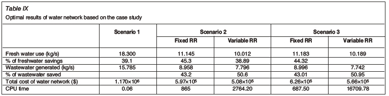
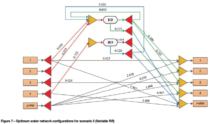
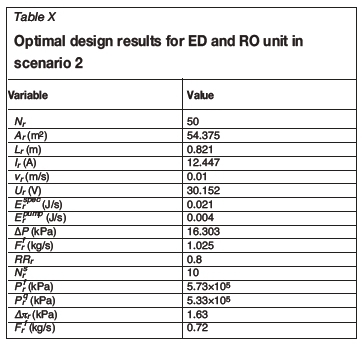
From the results in Table IX it is evident that the variable removal ratio in case 3 presents the optimal configuration, since the model is allowed to choose the performance parameters of the membrane regenerators. The results also show that incorporating multiple membrane regenerators with different performance and inlet and outlet contaminant limits in a water network can lead to an optimal use of fresh water. The inlet contaminant limits were set at different levels in order to allow the membrane regenerators various options for contaminant treatment. The variable removal ratio model in scenario 4.3 proves to be the optimal results for the case study as represented in Figure 7. The configuration showed that regeneration re-use and recycle within the water network between the regenerators resulted in a 44.3% reduction in fresh water consumption, 50.9% reduction in wastewater generation, and 45% savings in the total annualized water network cost as compared to case 1. Table X shows the design results of the ED and RO units respectively.

 

 

 

Conclusion

This work addresses the synthesis of a multi-membrane regeneration water network by proposing a water network model that incorporates detailed models of ED and RO regenerators. Different cases were considered under which the respective MINLP models were developed, and for each case a relevant literature case study was applied to demonstrate the applicability of the proposed model. Overall, the results showed that the use of a detailed model guarantees more accurate and reliable results in terms of water network synthesis as well as regenerator design. Savings of up to 44% in fresh water intake and reductions of up to 80% in wastewater generation and 45% in the total annualized cost were obtained. Additionally, because a detailed regenerator model presents an expression of the regeneration cost, it also gives optimal regenerator operating variables for minimal energy usage, thereby illustrating the inadequacy of the 'black-box' approach to superstructure optimization. Energy savings up to 82% were achieved. The results also showed an added advantage in setting the regenerator removal ratio as compared to fixing it arbitrarily. It is noteworthy that although the proposed models cater only for ED and RO regeneration technologies, they offer scope for future work, and the problem can be extended to incorporate other membrane technologies such as ultrafiltration, microfil-tration, and nanofiltration.

 

Nomenclature

Sets

J {j|j=water source}

I {i|i=water sink}

M {m|m=contaminants}

R {r|r=regeneration units}

Parameters

D^s_j,i Manhattan distance between source j and sink i

D^d_r,i Manhattan distance between regenerator r and sink, i D^y_r,rManhattan distance between regenerators r and r'

D^k_j,rManhattan distance between source j and regenerator

D_j^da_n Manhattan distance between source j and node n

ΔP_r^m Shell side pressure drop per module

P^p_r Pressure of a permeate stream from regenerator r

μ Solution viscosity

A Water permeability coefficient

A^f Annualization factor

a^LCD LCD constant

b^LCD LCD constant

C^chem Cost parameter for chemicals

C^elec Cost of electricity

C^FW Fresh water cost

C^mod Cost per module of HFRO membrane

C^pump Cost coefficient for pump

C^tur Cost coefficient for turbine

C^WW Wastewater treatment cost

F Faraday constant

k^el Cost of electricity

k^m Solute permeability constant

k^mb Cost of membrane

k^tr Conversion factor

LR_r Liquid recovery for regenerator r

m Interest rate per year

n Maximum equipment life

OS Proportionality constant between the osmotic pressure and average salt mass fraction on the feed side

p Parameter for carbon steel piping

q Parameter for carbon steel piping

S^m Membrane area per module

t^dOperating time per year

v Pipe linear velocity

w Cell width

z Valence

α Spacer shadow factor

β Volume factor

δ Cell thickness

ε Safety factor

ζ Current utilization

η Pumping efficiency

η^pump Pump efficiency

η^tur Turbine efficiency

λ Equivalent conductance

Λ° Infinite conductivity

ρ Total membrane resistance

σ,φ Limiting current density constants

γ Dimensionless constant

Continuous variables

TAC_r Total annualized cost for regenerator r

A_r Membrane area required by regenerator r

E_r^spec Specific desalination energy required by regenerator r

E_r^pump Specific pumping energy required by regenerator r

I_r Electrical current required by regenerator r

L_r Stack length

v_r Linear flow velocity at stage s

U_r Voltage applied

ΔP_r Pressure drop across the regenerator

F_f Regenerator feed flow rate

F_r^dil Final diluate stream flow rate of regenerator r

F_r^p Diluate stream flow rate for regenerator r

F_r^w Concentrate stream flow rate for regenerator r

F_r^cr Concentrate stream recycle flow rate for regenerator r

F_r^r Recycle stream flow rate for regenerator r

F_r^con Final concentrate flow rate for regenerator r

F^d_{r, i} Diluate flowrate to sink i

F^c_ri Concentrate flow rate to sink i

Fj Source flow rate

F^k_jr Flow rate from source j to regenerator r

F^Sj_{, i} Flow rate from source j to sink i

F_r^x_r' Recycle from diluate stream to regenerator feed

F_r^y_f Recycle from concentrate stream to regenerator feed

Fi^b Sink i flow rate requirements

C_r^f Regeneration feed concentration for regenerator r

C_r^wf Concentration of feed concentrate stream for regenerator r

C_r^cr Concentration of recycling concentrate for regenerator r

C_r^w Concentration of concentrate waste stream for regenerator, r

C_r^dil Diluate contaminant concentration

c_r^con Concentrate contaminant concentration

S_r^U Maximum allowable regenerator concentration

C_j Source concentration of

C_i^U Maximum allowable sink concentration

F_jn^da Allocated flow rate between sources j and node n

F^pe_r,i Flow rate of the permeate stream from regenerators r to sinks i

F_r^q_j Flow rate of the retentate stream from regenerators r to sinks i

F_n^a Flow rate of streams from re node n

P_n^a Pressure of streams leaving node n

P_nⁱ Pressure of an inlet stream to an energy recovery turbine from node n

P_n^o Pressure of an outlet stream from an energy recovery turbine from node n

P_r^q Pressure of a retentate stream from regenerator r

C_{r m}^av Average concentration of contaminant m in the high-pressure side of regenerator

C_r^f_m Concentration of contaminant m in the feed to the regenerator r

C_r,m^peConcentration of contaminant m in permeate stream leaving regenerator r

F_r^peFlow rate of permeate/diluate stream leaving the regenerator r

F_r^qFlow rate of retentate stream leaving the regenerator r

C_r^q_mConcentration of contaminant m in retentate stream leaving regenerator r

P^f_rFeed pressure into regenerator r

C^eqEquivalent concentration

FW Fresh water flow rate

i^pracPractical limiting current density

RR_rRemoval ratio for regenerator r

WW Waste water flow rate

ΔP_rPressure drop over regenerator r

Δπ_rOsmotic pressure on the retentate side of regenerator r

k Specific conductance

Λ Equivalent conductivity

 

Binary variables

 

 

 

Integer variables

N^s_rNumber of hollow fibre modules of regenerator r

N_rNumber of cell pairs per ED

 

Acknowledgement

The authors would like to thank the National Research Foundation (NRF) for funding this work under the NRF/DST Chair in Sustainable Process Engineering at the University of the Witwatersrand, South Africa.

 

References

Ahmetovic, E. and Grossmann, I.E. 2010. Strategies for global optimization of integrated process water networks. 20th European Symposium on Computer Aided Process Engineering - ESCAPE20. Pierucci, S. and Buzzi Ferraris, G. (eds). Elsevier.         [ Links ]

Alva-Argáez, A., Kokossis, A., and Smith, R. 1998. Wastewater minimization of industrial systems using an integrated approach. Computers and Chemical Engineering, vol. 22. pp. 741-744.         [ Links ]

Bagajewicz, M. and Savelski, M. 2001. On the use of linear models for the design of water utilization systems in process plants with a single contaminant. Waste Management, vol. 79. pp. 600-610.         [ Links ]

Bandyopadhyay, S. and Cormos, C.-C. 2008. Water management in process industries incorporating regeneration and recycle through a single unit. Industrial and Engineering Chemical Research, vol. 47. pp. 1111-1119.         [ Links ]

Chew, I.M.L., Tan, R., Ng, D.K.S., Foo, D.C.Y., Majozi, T., and Gouws, J. 2008. Synthesis of direct and indirect and interplant water and network. Industrial and Engineering Chemical Research, vol. 47. pp. 9485-9495.         [ Links ]

Doyle, S.J. and Smith, R. 1997. Targeting water reuse with multiple contaminants. Process Safety and Environmental Protection, vol. 75, no. 3. pp. 181-189.         [ Links ]

El-Halwagi, M. 1997. Pollution Prevention through Process Integration. Academic Press, San Diego.         [ Links ]

Rossiter, A.P. and Nath, R. 1995. Wastewater Minimization using Nonlinear Programming. McGraw-Hill.         [ Links ]

Salveski, M. and Bagajewicz, M. 2000. On the optimality conditions of water utilization systems in process plants with single contaminants. Chemical Engineering Science, vol. 55. pp. 5035-5048.         [ Links ]

Strathmann, H. 2010. Electrodialysis, a mature technology with a multitude of new applications. Desalination, vol. 264. pp. 268-288.         [ Links ]

Takama, N., Kuriyama, T., Shiroko, K., and Umeda, T. 1980. Optimal planning of water allocation in industry. Computers and Chemical Engineering, vol. 4, no. 80. pp. 251-258.         [ Links ]

Tan, R.R., Ng, D.K.S., Foo, D.C.Y., and Aviso, K.B. 2009. A superstructure model for the synthesis of single-contaminant water networks with partitioning regenerators. Process Safety and Environmental Protection, vol. 87, no. 9. pp. 197-205.         [ Links ]

Tawarmalani, M. and Sahinidis, N.V. 2005. A polyhedral branch-and-cut approach to global optimization. Mathematical Programming, vol. 103, no. 2. pp. 225-249.         [ Links ]

Tsiakis, P. and Papageorgiou, L.G. 2005. Optimal design of an electrodialysis brackish water desalination plant. Desalination and the Environment, vol. 173, no. 2. pp. 173-186.         [ Links ]

Yang, L., Salcedo-Diaz, R., and Grossmann. E.I. 2014. Water network optimization with wastewater regeneration models. Industrial and Engineering Chemistry Research, vol. 53. pp. 17680-17695.         [ Links ]

Wang, Y.P. and Smith, R. 1994a. Wastewater minimization. Chemical Engineering Science, vol. 49, no. 94. pp. 981-1006.         [ Links ]

Wang, Y.P. and Smith, R. 1994b. Design of distributed effluent treatment systems. Chemical Engineering Science, vol. 49, no. 94. pp. 3127-3145.         [ Links ]

Wright, M.R. 2007. An Introduction to Aqueous Electrolyte Solutions. Wiley, Chichester, UK.         [ Links ]

 

 

Paper received May 2015.