Application of the attainable region technique to the analysis of a full-scale mill in open circuit

 

 

F.K. Mulenga^I; M.M. Bwalya^II

^IDepartment of Electrical and Mining Engineering, University of South Africa
^IISchool of Chemical and Metallurgical Engineering, University of Witwatersrand, South Africa. © The Southern African Institute of Mining and Metallurgy, 2015

 

 

---

SYNOPSIS

The application of the attainable region (AR) technique to the analysis of ball milling is currently limited to batch data. This paper introduces the use of the technique to continuous milling. To this end, an industrial open milling circuit processing a platinum ore was surveyed. Samples were collected and later characterized by means of laboratory batch testing. On site, several milling parameters were varied systematically so as to collect data for modelling purposes. These paramters included ball filling, slurry concentration, and feed flow rate. After data analysis, a simulation model of the open milling circuit was developed under MODSIM^®, a modular simulator for mineral processing operations. The mill was then simulated and the data generated was analysed within the AR framework. Initial findings reveal an opportunity to gain valuable insight by studying milling using the AR technique. From an exploratory perspective and inasmuch as this study is concerned, feed flow rate, ball size, and ball filling were identified as being pivotal for the optimization of open ball-milling circuits. Mill speed, on the other hand, had only a limited effect on the production of particles in the size range -75 +10 μm.

Keywords: attainable region, ball milling, population balance model, milling parameters, scale-up procedure, MODSIM® simulator

---

 

 

Introduction

Glasser and Hildebrandt (1997) propounded the attainable region (AR) as a technique for the analysis of chemical engineering reactor systems. Results have since been produced and tested on both the laboratory and pilot scales. The method results in a graphical description of chemical reactions by considering the fundamental processes taking place in the system, rather than the equipment. From the plotted graphs, the process and the reactors can be synthesized optimally into a flow sheet.

The use of the AR method still has a long way to go as far as mineral processing is concerned. For instance, several articles have reported the application of the AR technique to ball milling: Khumalo et al. (2006, 2007, 2008); Khumalo (2007); Metzger et al. (2009, 2012); Metzger (2011); Katubilwa et al. (2011); Hlabangana et al. (2012). Their main shortcoming has been the exclusive use of laboratory batch grinding data.

To address this deficiency, Mulenga and Chimwani (2013) proposed a way by which the technique could be extended to continuous milling. In effect, the batch milling characteristics of a platinum-bearing ore (Chimwani et al., 2013) were used and scaled up to an open milling circuit. Then, with simplifying assumptions, an attempt was made to optimize the residence time of particles inside the mill. Later, Chimwani et al. (2014a) presented some optimization examples involving various milling parameters. The sequence of published articles then paved the way for the study of industrial milling systems with the AR methodology.

Admittedly, the limitation has been that the exit classification of the milling circuit was not included (Mulenga and Chimwani, 2014; Chimwani et al., 2014a, 2004b). The importance of this internal phenomenon has been discussed in detail elsewhere (Cho and Austin, 2004; Austin et al., 2007). Suffice to say that the exit classification (also referred to as post-classification or internal classification) is responsible for the preferential discharge of smaller particles and the retention of larger particles back into the mill load until sufficient milling has been achieved.

In the present work, MODSIM® - a modular software package for the simulation of mineral processing units (King, 2001) - was used. The flexibility of the simulator enabled the internal classification of particles before exiting the mill to be taken into account, thereby making it possible to generate industrially sound data. From there, the effects of ball filling, ball size, mill speed, and feed flow rate on the product of an open milling circuit were simulated.A methodology for the application of the AR technique to realistic open mill models is presented and illustrated using the simulated data. The AR profiles produced are analysed and interpreted within the AR framework. As a result of this analysis strategy, new insights on open milling circuits are brought to light and discussed. Finally, recommendations for future work are formulated.

 

Theoretical background

This section reviews the theoretical modelling of batch milling as well as the fundamental processes associated with milling in general. The basic concepts underpinning the AR technique are also discussed.

Ball milling model

The objective of any comminution operation is to break large particles down to the required size. In tumbling ball mills, this is achieved through repetitive breakage actions. Fragments from each particle generated after the initial breakage actions generally fall into a wide range of sizes. However, some of the daughter fragments are still coarse and require further breakage. That is why the milling process can be regarded as the combination of two simultaneous actions: the selection of particles for breakage, and the actual breakage resulting in a particular distribution of fragment sizes after the particle has been selected (Gupta and Yan, 2006). A size-mass balance inside the mill that takes into account the two aforementioned reactions eventually results in the full description of the grinding process.

Let us consider particles of size x_iat time t within a given feed size distribution; denote their mass fraction w_i(t). Now, take a time interval dt small enough to allow only single breakage events to occur on a fraction of w_i(t).

If the fraction selected for single event breakage per unit time is S_I, then S_i.dt represents the mass fraction broken after the time interval dt. This mass breaks into a wide range of child particles, the size of which spans from the parent size xi down to x_n.

In an open ball-milling circuit, the flow of material in and out of class interval [x_i, x_i+1] can be divided into four categories: the mass fraction accumulated because not selected for breakage, the mass fraction leaving the class interval as a result of the single breakage events, the incoming mass fraction through breakage of particles larger than xi, and the incoming mass fraction from the new feed.

After time interval dt, the second category of particles is given by Si.dt, while the third category necessitates the determination of the mass fraction reporting to [x_i, x_i+1] as a result of the breakage of selected particles of initial sizes larger than x_i.

The term Si is the selection function; it represents the rate of breakage of particles of size x_i. Austin et al. (1984) proposed the following empirical model to express the variation of the selection function with particle size:

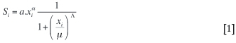
where

x_iis the upper size of the particle size interval i under consideration

a and μ are parameters that are mainly functions of milling conditions

α and Λ are material-dependent parameters.

Let us now assume that xj represents any particle size larger than x_i(that is, x_n < x_i < x_j). It is clear that the particles of size xjselected for breakage will give birth to particles of sizes spanning from x_j down to x_n.

Because particle size is conventionally measured using a series of sieves with mesh apertures arranged in a geometric sequence (generally 2^1/2or 2^1/4), a convenient notation will be introduced whereby the largest size class interval is named x₁. Particles in this class pass through a sieve of size x₁ but are retained on a sieve of size x₂. Consequently, the mass fraction of particles falling in size class interval [x₁, x₂], or in class 1 for short, at time t becomes w₁(t). The last size class interval, known as the 'sink' and composed of the smallest particles, is termed [xn, 0] or class n. Particles in the sink class are therefore of size xn and their corresponding mass fraction is w_n(t).

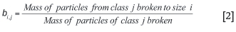
In order to define the breakage function, consider two class intervals [x_i, x_i+1] and [xj xj+₁] containing particles of size x_iand xj respectively where x_i< xj. The breakage function, better called the primary breakage distribution function, can be defined as the average size distribution resulting from the fracture of a single particle (Kelly and Spottiswood, 1990). It is used to describe the size distribution of the child particles produced after a single step of breakage of a parent particle of the material under consideration. Hence, if a parent particle is impacted by a grinding ball, the resulting product will consist of broken particles in a wide size range. The description of this breakage event (single step of breakage) is made possible by defining the breakage function of the material being broken. To this end, the primary breakage distribution function of particles of size xjbreaking into size xi is defined as follows:

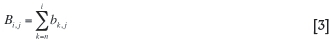
A more convenient way of describing the breakage distribution function is to use the cumulative breakage function, defined as follows (Austin et al., 1984):

With this new definition, the following empirical model relating the cumulative breakage function to particle size can be used (Austin et al., 1984):

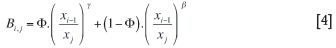
where

β is a parameter characteristic of the material used

γ is also a material-dependent characteristic

Φ represents the fraction of fines produced in a single fracture event. It is also dependent on the material used.

Attainable region analysis applied to ball milling

The AR methodology was intended primarily for chemical process optimization. That is why its original utilization entailed the concentrations of reactants and products of interest. In milling, however, particles break into different size classes. Hence, by analogy between chemical reactions and milling, size classes can be regarded as chemical species. In doing so, the feed size class becomes the reactant and the undersized classes are the products of the breakage reaction.

Glasser and Hildebrandt (1997) define the attainable region as 'the set of all physically realizable outcomes using only the processes of reaction and mixing in steady-state systems for some given feed(s)'. In other words, given the feed and the reaction kinetics, the set of all possible outputs of a chemical reaction can be determined; and from there, the best operating conditions (subject to some external constraints) can be deduced.

In order to illustrate the paradigm, let us start off with a narrow-sized feed material [x₁ < x < x₂]. If after batch-milling the feed sample for a grind time t = 1 minute, a complete particle size analysis is performed from x1 down to x_n, Figure 1 can be plotted.

 

 

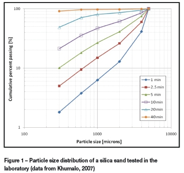
Figure 1 does not only present the product size distribution (PSD) for t = 1 minute, but also shows the PSDs corresponding to grinding times ranging from 2.5 to 40 minutes for which particle size analyses were performed in a similar fashion.

Let us consider a given passing sieve size x_k, where x_kε {x_iwith 1 < i < n}, and define new size classes:

> The feed size class or the material of size x falling between x₁ and x₂; the mass fraction of material in this class will be termed m₁

> The middling size class constituted of particles of size x between x₂and x_k; the corresponding mass fraction will be termed m₂

> The fines size class m₃, which is defined as the mass fraction of material passing through screen size x_k.

For illustration purposes, let x₂ and x_kbe 4000 μm and 600 pm respectively. The change in mass fraction in each new size class (i.e. m₁, m₂, and m₃) can now be tracked as a function of grinding time: this will look something like Figure 2.

 

 

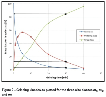
If the objective is, say, to produce as much material in the middling class as possible, grinding the feed for 5 minutes would be the way to go, as shown in Figure 2. Note that a model is not required to find such an optimum; instead, a straightforward exercise of interpreting and reading graphs does the work.

From the mass fraction profiles reported in Figure 2, let us present the data in the last format, which is of much interest to the AR technique. In order to perform the transformation, respective mass fractions are read off from Figure 2 at grinding time t = 30 minutes. They are then mapped onto a two-dimensional mass fraction space, that is, (m₁, m₂). By repeating the process and mapping all the data points in Figure 2, the AR plot is produced as shown in Figure 3. This figure presents the same data produced from the silica sand material in Figure 2, but this time in the two-dimensional space (m₁, m₂).

 

 

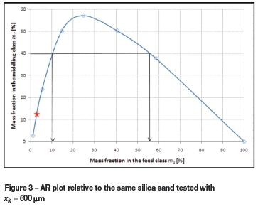
It should be recalled that m₃ can be inferred by mass balance at any stage of the process. Most importantly, Figure 3 represents the path followed by the milling process to achieve the specified objective function from the system feed. This is referred to as the 'attainable region path'.

The star marker on the plot (in Figure 3) corresponds to the 30 minutes' grinding time considered earlier. From an AR perspective, one would say that about 97% of the feed is needed to produce approximately 13% of middling; and this, after 30 minutes of grinding. It is therefore understood that after 30 minutes only 3% mass fraction is left in the feed class m₁while 13% of middling m₂ is produced.

If the objective is to produce at least 40% of m₂, the AR plot indicates that between 44% and 89% of the feed material is required. The graph shows that, for the objective to be met, between 11% and 56% of the material should remain in class m1. This translates to a mass fraction of between 89% and 44% of material that needs to be ground out. Nonetheless, information such as the specific energy to be used, or some other operating constraints, will orientate the process engineer towards the choice of the right mass fraction to be milled.

It appears that AR paths make it possible to characterize the selectivity of the process. In other words, it is possible to determine the fraction of initial feed material that will report to the size class of interest under given operating conditions.

It is important to note that the AR analysis presented here is for illustration purposes, and that each case study will require particular attention.

The last point to discuss is the idea behind the term 'attainable region'. This can be conceived as follows. In Figure 4 (created from Figure 2), point A represents a fresh feed not yet ground, while point B represents a product milled for some time that consists of 15% m1 and 50% m2. It is possible to mix a fraction of A, say 25%, and combine it with 75% of B to obtain a composite material C. One can carry on with this exercise and fill up the region between the AR plot and the x-axis with data points for different combinations. The data points will represent all the possible composite materials that can be obtained from the milling system using the mixing principle. That is why the stripped region in Figure 4 is called the attainable region.

 

 

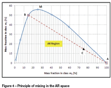
If the AR region is concave (note that the striped region in Figure 4 is convex), mixing presents an advantage in that more material can be produced in addition to that generated by the grinding process itself. Furthermore, the maximum point M (in Figure 4) can be achieved only if the class of interest is defined with upper and lower screen size boundaries. As a corollary to this, the sink fraction (i.e. class n) and the feed fraction (i.e. class 1) never experience such a maximum. That is the reason why a definite class interval is always required for process optimization, and not a semi-infinite class. Sink and feed fractions are typical examples of semi-infinite classes.

 

Data collection methodology

This article aims to present a way of applying the AR technique to an open milling circuit. To this end, a full-scale mill, as well as the ore being processed, were characterized. The data collection technique is discussed in the subsequent sections, together with the technological specifications of different experimental set-ups. The simulation package employed in the modelling of the full-scale mill is also presented succinctly. Finally, the input parameters for the actual ball mill model are listed.

Full-scale milling data

The full-scale mill considered in this work is an overflow discharge mill, run in open circuit and used in the secondary milling of a UG2 platinum ore. The technological and operating specifications are:

Mill rated power 11 000 kW

Mill full length L = 9.6 m inside liners

Mill diameter D = 7.312 m inside liners

Mill speed φ_C= 75% of critical

Ball filling J ranging from 25% to 33%

Steel ball diameter d = 40 mm.

The mill is lined with 44 rubber lifters that have a height of 100 mm. The solids concentration in slurry is on average 75% by mass for a solids feed rate, F, of 330 t/h.

The set of industrial parameters that were monitored is shown in Figure 5, together with the flow sheet of the secondary milling section. Data on the density, the flow rate, and the size distribution of the densifier underflow stream was collected at the mill inlet, as well as the flow rate of the mill dilution water. At the mill discharge, the density, flow rate, and size distribution of the mill product were measured.

In this work, the aforementioned industrial data was used to validate the simulation model of the open milling circuit in Figure 5. It is important to mention that the full-scale milling data collected was the result of a fruitful collaboration between Magotteaux (Pty) Ltd, the University of Cape Town (UCT), Anglo Platinum's Waterval UG2 Concentrator, and the University of the Witwatersrand (Wits). More details on the industrial campaign and the sampling set-up are provided in Keshav et al. (2011).

Batch milling data

The complete description of milling necessitates an accurate measurement of all parameters involved in the process model. A good way of doing this is to run well-planned batch tests on mono-sized feed samples using the one-size-fraction method (Austin et al., 1984). In this method, a sample in one size class is prepared and loaded in a small laboratory mill together with grinding balls. Milling is performed for several suitable grinding time intervals. After each interval, the product is sieved, returned to the mill, and then further milled. In this way, the mill product is monitored for the different grinding time intervals chosen a priori. Lastly, laboratory results are analysed in order for the selection function parameters (i.e. a_T, μ_T, α, and Λ in Equation [1]), as well as the breakage function parameters (i.e. β, γ and Φ in Equation [4]), to be determined. That is why the primary objective of batch grinding tests is to measure the milling characteristics of a material under given experimental conditions.

In the present work, the material used in the batch testing programme was the platinum-bearing UG2 ore already subjected to primary milling. The UG2 is one of the platinum-rich layers in the Bushveld Complex (BC) of South Africa and accounts for about 60% of South Africa's platinum reserves.

Internal references from the Waterval concentrator reported that the specific density of the UG2 ore used is 3.47 kg/cm3 as established in routine inspection. The ore supplied was a fine material of size less than 1700 μm.

Batch testing was conducted on three mono-sized ore samples: -850 +600 μm, -600 +425 μm, and -425 +300 μm. Three ball diameters were used: 10 mm, 20 mm, and 30 mm. The feed samples were dry batch-milled for 0.5, 1, 2, 4, 8, 15, and 30 minutes. After each grinding time, a representative sample was taken from the mill powder for conventional sieving. In total, nine series of batch tests were carried out for seven grinding times.

Table I lists the breakage function and selection function parameters characterizing the UG2 ore used. Chimwani et al. (2013) discussed in detail how these parameters were determined.

 

 

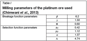
The values in Table I were measured under the following experimental conditions: ball diameter d_T= 20 mm; ball filling J_T= 20%; powder filling U_T= 0.75; mill speed Ø_ct= 75% of critical; and mill diameter DT = 302 mm. All this information was used in setting up the simulation model for the open milling circuit in Figure 5.

If one considers a ball mill of internal volume Vmill, it is clear that the mill can theoretically carry an equal volume of grinding media to its own volume. In practice, however, only a fraction of the volume, Vballs, is occupied by grinding balls. The ratio of the volume occupied by balls at rest to the mill volume is defined as the ball filling, J.

In addition to the bed of balls, and specifically in wet milling, slurry (which is a mixture of ore particles and water) is also loaded into the mill. Depending on the volume loaded, slurry occupies firstly the interstices between the grinding balls before immersing the bed of balls at rest. The ratio of the volume of slurry loaded to the volume of ball interstices available within the bed at rest is the slurry filling, U. Hence, considering a ball filling J, the volume of slurry Vsl needed to achieve slurry filling U is determined as follows:

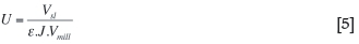
where ε represents the porosity of the bed of grinding media at rest, which is assumed to be 0.4 on average.

A limitation to the gradual increase in ball filling is that the maximum power occurs when the media filling, J, is at approximately 45% of the mill volume; after that, power tends to decrease. By the same token, slurry should preferably be loaded in a way that ensures that most of the material is held in the media interstices (Latchireddi and Morrell, 2003). Otherwise, if the level of slurry is low, the charge is more likely to experience ball-to-ball contact and waste energy. On the other hand, if there is more slurry than the media charge can hold within, a pool of slurry will form, with impact breakage becoming less pronounced.

Another important milling parameter that needs a brief explanation is the rotational speed. Mill speed is commonly defined as a fraction of the theoretical critical speed of the mill. The critical speed is the speed of the mill at which a single ball starts to centrifuge. At this speed, the grinding ball sticks against the mill wall because the centrifugal and the gravitational forces are in balance. Critical speed is given in revolutions per second by the following expression:

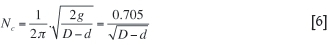
where

D is the internal diameter of the mill

d is the diameter of the grinding ball under consideration

g is the gravity constant, i.e. 9.81 m/s².

Therefore, if the mill is said to run at 70% of critical, this simply means that the actual speed of the mill, expressed in revolutions per second, is 70% of the theoretical critical speed calculated using Equation [6].

MODSIM®, the modular simulator

The core of the investigative work was centred on the use of the academic version 3.6 of MODSIM®, a specialized steady-state simulator. The software package is a modular simulator for ore-dressing plants. King (2001) provides a comprehensive review of all the unit processes available in MODSIM^® as well as a description of relevant models applicable to each operation.

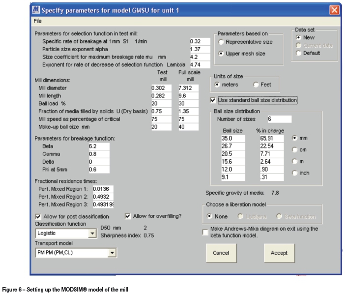
As far as the milling circuit model is concerned, GMSU was found to be the adequate option for this exploratory study. The MODSIM® ball mill model is an encapsulation of the scale-up procedure by Austin et al. (1984). It is used when the selection function and breakage function parameters have been determined from laboratory batch tests. In addition to this, the dimensions of the full-scale mill should be available. This is indeed the case in the present work. Most importantly, the GMSU model assumes that post-classification is present and that the mill load is perfectly mixed.

Figure 6 shows the form for the input of parameter values necessary to the GMSU model. In this study, no liberation model was considered; furthermore, provision was made for mill overfilling.

In the execution of all simulations, unless otherwise stated, the standard ball size distribution available in MODSIM® and the feed size distribution in Figure 7 were used.

 

 

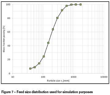
Figure 7 represents an average feed size distribution calculated from the various feed samples collected on the plant during the sampling campaign described previously.

 

Simulation results

Simulation model validation

This section presents the develoμment of the MODSIM^® ball milling model as well as aspects of the model validation undertaken. The effects of selected milling conditions are discussed in subsequent sections.

As a starting point, a simulation program for the open milling circuit in Figure 5 was initiated using MODSIM^®. To this end, the breakage characteristics of the ore (see Table I) were declared for scale-up as shown in Figure 6. The product size distributions were then generated for different operating conditions.

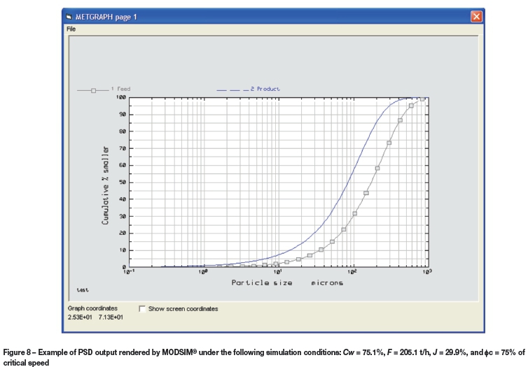
Figure 8 illustrates a typical simulation output window rendered by MODSIM^®.

Thereafter, the AR methodology was applied to the data with the objective of assessing the influence of several milling conditions on the production of material amenable to flotation from the initial feed size distribution shown in Figure 7. The product class m2 was set between 75 μm and 9 μm because the platinum industry in South Africa generally requires the product to be below 75 μm before it is sent to flotation. The cut-off size of 9 μm was guided by the poor flotation performance reported for particles less than 10 μm on average (Rule and Anyimadu, 2007).

All in all, the initial feed class m₁ considered was -1700 +75 μm, while the objective function was to explore the production of m2, i.e. -75 +9 μm, as a function of ball filling, feed flow rate, mill speed, and ball diameter.

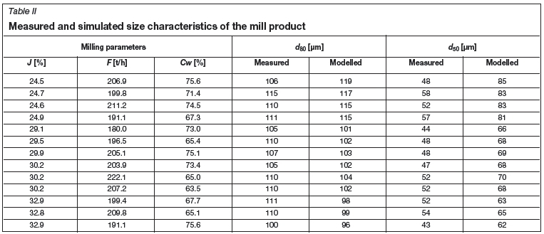
Before reporting the findings pertaining to the AR method, simulated results from the MODSIM® milling model were compared to the industrial data. It can be seen in Figure 9 that model and measurement agree well for particle sizes larger than 100 μm. In contrast, below this size, measurements are under-predicted by the simulation model. The model predicts a coarser mill product compared to the industrial data.

 

 

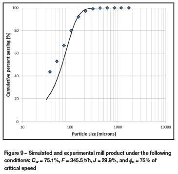
This is also evident in Table II, in which the predicted 50% passing sizes (d₅₀) are higher than the experimentally measured ones. Possible reasons for these discrepancies are presented later in the Discussion section. However, agreement on the 80% passing size (d₈₀) is deemed enough (see Table II) to carry out exploratory simulations and meet the objectives set for the present article.

Effects of ball filling on mill throughput

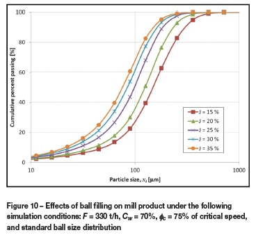
In the first set of simulations, the effect of ball filling on the mill throughput was assessed. Four levels of ball filling were simulated: J = 10, 20, 30, and 40%. The term 'throughput' is used to refer solely to the mass fraction of particles in class m2 present in the mill product. It is an indication of the ability of the mill to produce the desired particles, i.e. -75 +9 μm. It does not consider the mass or volume flow rate of the mill discharge stream.

It can be seen in Figure 10 that the mill product size distribution becomes finer as ball filling is increased. Note here that feed flow rate, ball size distribution, slurry filling, and mill speed were kept constant.

 

 

Now, examination of the data in Figure 10 from an AR point of view reveals that the production of m2 follows a straight line which is close to the ideal AR profile. In effect, the ideal AR profile is represented in Figure 11 by the red dotted line: along this line, the feed is milled in such a way that the product reports to class m2 only. In other words, there is no loss to finer sizes or no material is produced below 10 μm.

 

 

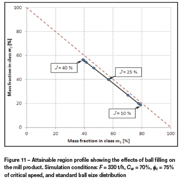
Because the AR plot in Figure 11 is close to the ideal AR plot, it can be argued that the effect of ball filling as far as the platinum ore and the full-scale mill set-up are concerned is such that particles are preferentially broken into m2. Three data points are also labelled to assist with the graphical interpretation.

Note that the identification of the optimum ball filling is not straightforward from Figure 11. However, it becomes easy to see the optimum once the data is presented using ball filling as the independent variable (see Figure 12).

 

 

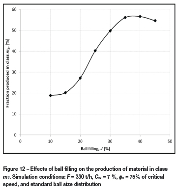
In addition to the above, the simulation results suggest that the optimum ball filling is somewhere between J = 35% and J = 40% as shown in Figure 12. In this range, the production of m₂ is as high as 56.5%.

Effects of feed flow rate on mill throughput

In the second set of simulations, the effect of solids feed rate was analysed while keeping ball filling, slurry filling, and mill speed constant.

For the sake of exploring the relevance of the AR technique, the flow rate was varied between 10 t/h and 400 t/h. It can be seen in Figure 13 that although the full-scale mill has been operated at a flow rate of the order of 300-400 t/h, better throughput may be obtained at flow rates as low as 30 t/h. Furthermore, the mass fraction of m2 in the mill product increases from an average of 40% to in excess of 75%. This is indicative of the fact that lower flow rates are conducive to the production of -75 +10 μm particles. Vermeulen et al. (1991) reported similar findings using mills of different sizes in open circuit. The only difference is that the target product size was less than 75 μm. The present work, on the other hand, focuses on particles between 75 μm and 10 μm.

 

 

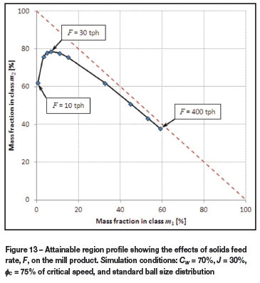
Most importantly, even though a better mill product is obtained at low flow rates, the volume produced may be too low to justify the implementation of the AR optimum. A study is currently underway to find a reasonable trade-off.

Effects of mill speed on mill throughput

The next series of simulations was aimed at investigating the effect of mill speed on the production of m2. The mill speed values considered spanned from 50% to 90% of critical speed.

Similarly to the effect of ball filling examined previously, the AR profile in Figure 14 indicates a limited effect of mill speed on the throughput. However, presenting the production of m2 as a function of mill speed proves to be insightful. Indeed, Figure 15 shows an increase in m2 with mill speed until 80% of critical speed; then a steady drop follows.

 

 

 

 

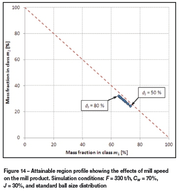
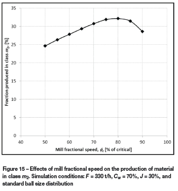
Figure 15 also suggests that in order to obtain maximum production of m2, mill speed should be adjusted to about 80% critical. The optimum operating range as far as m2 is concerned is therefore 75-85% of critical speed.

Effects of ball size on mill throughput

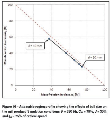
The last of series of simulations sought to ascertain the effect of ball diameter on mill throughput. To this end, the diameter of grinding balls was varied between 10 mm and 50 mm.

It can be seen in Figure 16 that smaller grinding balls encourage the production of m2 while larger ones basically break particles indiscriminately. The problem with smaller balls is that their life span inside the mill is short, and therefore, makes their use less recommendable. That is why it is believed that a ball mix with a high proportion of small balls would be a viable option (Cho etal., 2013). The mixture of balls will take advantage of the number of small balls while extending their life with a fair amount of larger ones.

 

 

 

Discussion

Attempts to apply the AR technique to comminution have been undertaken in the past with interesting outcomes. In particular, a viable approach has been proposed (Mulenga and Chimwani, 2013; Chimwani et al., 2014a, 2014b) and is being further developed. The shortcoming of this series of articles has been the exclusion of the internal classification at the mill exit.

Unlike the previous papers, the present work has utilized a software package that is able to simulate open milling circuits while allowing for exit classification. It has thus been possible to generate sound industrial data for analysis within the AR framework. Nonetheless, the simulation needed validation before use. The outcomes are shown in Figure 9 and Table II.

As an exploratory study, it is argued that the simulation model is able to predict satisfactorily the 80% passing size (d₈₀) of the mill product. However, the 50% passing size ( d₅₀) was over-predicted. One possible reason for the systematic discrepancies observed is believed to be related to the modelling of the internal classification. Indeed, the general consensus is that the exit classification is predominantly a function of particle size (Austin et al., 1984; King, 2001; Napier-Munn et al., 1996; Cho and Austin, 2004; Cho et al., 2013). One of the widely used models for the exit classification is the logistic function given in Equation [7] (Austin et al., 1984):

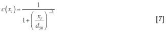
where

x_iis the upper size of the particle size interval i under consideration

d₅₀ represents the cut-off size of the post-classification. It can be regarded as the size at which particles have equal chance of reporting to the mill product or back into the mill load. Thus, c(d₅₀) = 0.5

λ is a parameter defining the gradient of the classification function c(x_i) when plotted as a function of particle size x_i. The gradient is related to the sharpness index S.I. as follows:

In the MODSIM^® model of the mill, the following classification parameters were found to produce good results: d50 = 128.6 μm and S.I. = 0.35.

To return to the discrepancies in Figure 9, one can see that Equation [7] is intrinsically dependent on particle size xi. It is possible that the actual exit classification of the mill could be affected by operating parameters other than particle size. If that is the case, then the classification model should be revised and the predicted mill product adjusted. Work is currently being conducted in which the classification function is revisited to include milling parameters such as ball filling and slurry concentration. Once this is done, an improved classification model that allows for milling parameters will be used instead of the particle-size-based classification function in Equation [7]. The direct implication will be a robust simulation model with improved prediction abilities.

This brings us to discuss the effect of the first milling parameter investigated, that is, ball filling.

The observed trend was that increased ball fillings yielded a higher production of m2; however, ball fillings above J = 40% brought about the opposite effect. This is consistent with the observation that wet mills are efficient when slurry completely occupies the interstices between the grinding balls (Latchireddi and Morrell, 2003; Tangsathitkulchai, 2003). In this case, the slurry filling of the mill is equal to unity (i.e. U = 1). Keshav et al. (2011) also reported similar findings, with an improved reduction ratio being noted when ball filling was increased. However, their target was the production of <75 μm and not m₂(i.e. -75 +10 μm) as is the case in the present work.

On another note, Mulenga and Chimwani (2013) were able to demonstrate that for an overflow discharge mill such as the one currently under consideration, a ball filling of J = 35% represents a threshold beyond which the slurry pool disappears. In other words, J = 35% approximately corresponds a slurry filling U = 1. That is ostensibly why in Figure 12 the optimum mill throughput is recorded at ball filling J = 35-40%.

As far as the second milling parameter is concerned, Figure 13 shows that a higher mass fraction of m2 is produced when the solids feed rate is decreased from 400 t/h to approximately 30 t/h. At feed rates less than 30 t/h, the proportion of m2 in the mill product falls sharply. This behaviour could be attributed to the fact that low flow rate implies a longer residence time of particles inside the mill, and therefore higher grinding levels. However, a much lower flow rate translates into a finer grind, which eventually results in particles reporting predominantly to size class m₃ ( i.e. -10 μm) and not m2, hence, the sudden drop in throughput.

Next, the effect of mill speed on the production of m2 is linked to the change in load behaviour of the mill. Indeed, a low mill speed is synonymous with low ball-to-ball and ball-to-ore impact levels inside the mill. Similarly, a very high mill speed incurs more particle centrifuging, and therefore less impact breakage. So, by and large, speeds of the order of Ø_c = 70-85% of critical ensure a high level of impact breakage and consequently a better grind (see Figure 15).

Lastly, based on the simulation results of the effect of ball size (see Figure 16), grinding balls of diameter d = 10 mm produced almost three times the m2 that was recorded with ball diameter d = 50 mm. This is ascribed to the fact that small balls are known to produce a finer grind (Austin et al., 1984; Katubilwa and Moys, 2009; Cho et al., 2013). They will therefore produce a higher fraction of m2 than larger grinding balls. Notwithstanding this, the life span of the small balls is short, and a mixture of balls of different diameters may be a better option. A study is currently in progress aiming at determining the best ball mix for the production of m₂.

 

Conclusion and future outlook

The main objective of the present work was the proposal of an attainable region (AR) framework for the analysis of open milling circuits.

Following the successful use of the AR technique, it is fair to state that the method has grown to becoming an alternative tool for the analysis of full-scale milling data. However, for the tool to be effectively used, one should rely on the classical milling model and build a robust simulator validated against industrial data. Once this is done, simulation data can be generated for analysis and optimization following the methodology proposed in this article.

Future studies will examine the effects of slurry density on milling. Energy usage for ball milling will also be included in the AR analysis. The possibility of generalizing the method to encompass closed milling circuits will also be considered. Equally important is the holistic integration of downstream concentration processes such as flotation with ball milling. This, of course, is dependent on a better characterization of the flotation performance of the ore.

Until all the above is addressed, it can be stated that the present exploratory work has demonstrated the suitability of the AR technique for studying open ball milling-circuits.

 

Acknowledgements

The authors are indebted to the University of South Africa (UNISA) and the University of the Witwatersrand for encouraging the collaborative work between the two institutions.

The industrial data used for validation purposes was the product of successful collaboration between Anglo Platinum, Magotteaux, the University of Cape Town, and the University of the Witwatersrand.

Special thanks to the Waterval Mine of Anglo Platinum for granting access to the plant, and also for technical support in setting up the experimental programme.

Appreciation is further extended to Dr Chris Rule, Head of Concentrator Technology at Anglo Platinum, for giving clearance to publish the paper as well as the industrial data collected at the Waterval Mine.

Magotteaux (Pty) Ltd, the developer of the specialized sensor Sensomag® used during the sampling campaign, is also acknowledged for the invaluable data extracted from their sensor. This information was critical in obtaining accurate estimates of grinding ball filling.

 

References

Austin, L.G., Julianelli, K., de Souza, A.S., and Schneider, C.L., 2007. Simulation of wet ball milling of iron ore at Carajas, Brazil. International Journal of Mineral Processing, vol. 84, no. 1-4. pp. 157-171.         [ Links ]

Austin, L.G., Klimpel, R.R., and Luckie, P.T. 1984. Process Engineering of Size Reduction: Ball Milling. Society of Mining Engineers of the AIME, New York.         [ Links ]

Chimwani, N., Glasser, D., Hildebrandt, D., Metzger, M.J., and Mulenga, F.K. 2013. Determination of the milling parameters of a platinum group minerals ore to optimize product size distribution for flotation purposes. Minerals Engineering, vol. 43-44. pp. 67-78        [ Links ]

Chimwani, N., Mulenga, F.K., Hildebrandt, D., Glasser, D., and Bwalya, M.M. 2014a. Scale-up of batch grinding data for simulation of industrial milling of platinum group minerals ore. Minerals Engineering, vol. 63. pp. 100-109.         [ Links ]

Chimwani, N., Mulenga, F.K., Hildebrandt, D., Glasser, D., and Bwalya, M.M. 2015. Use of the attainable region method to simulate a full-scale ball mill with a realistic transport model. Minerals Engineering, vol. 73, pp. 116-123.         [ Links ]

Cho, H. and Austin, L.G. 2004. A study of the exit classification effect in wet ball milling. Powder Technology, vol. 143-144. pp. 204-214.         [ Links ]

Cho, H., Kwon, J., Kim, K., and Mun, M., 2013. Optimum choice of the make-up ball sizes for maximum throughput in tumbling ball mills. Powder Technology, vol. 246. pp. 625-634.         [ Links ]

Glasser, D. and Hildebrandt, D. 1997. Reactor and process synthesis. Computers in Chemical Engineering, vol. 21, suppl. 1. pp. S775-S783.         [ Links ]

Gupta, A. and Yan, D.S. 2006. Mineral Processing Design and Operation: An introduction. Elsevier, Perth.         [ Links ]

Hlabangana, N., Vetter, D., Metzger, M.J., Glasser, D., and Hildebrandt, D. 2012. Industrial application of the attainable region analysis to a joint milling and leaching process. Proceedings of the VIII International Comminution Symposium - Comminution '12, Cape Town, South Africa. Minerals Engineering International, Falmouth, UK.         [ Links ]

Katubilwa, F.M. and Moys, M.H. 2009. Effect of ball size distribution on milling rate. Minerals Engineering, vol. 22, no. 15. pp. 1283-1288.         [ Links ]

Katubilwa, F.M., Moys, M.H., Glasser, D., and Hildebrandt, D. 2011. An attainable region analysis of the effect of ball size on milling. Powder Technology, vol. 210, no. 1. pp. 36-46.         [ Links ]

Kelly, E.G. and Spottiswood, D.J. 1990. The breakage function; what is it really? Minerals Engineering, vol. 3, no. 5. pp. 405-414.         [ Links ]

Keshav, P., de Haas, B., Clermont, B., Mainza, Α., and Moys, M.H. 2011. optimisation of the secondary ball mill using an on-line ball and pulp load sensor - the sensomag. Minerals Engineering, vol. 24. pp. 325-334.         [ Links ]

Khumalo, N. 2007. The application of the attainable region analysis in comminution. PhD thesis, University of the Witwatersrand, Johannesburg.         [ Links ]

Khumalo, N., Glasser, D., Hildebrandt, D., and Hausberger, B. 2008. Improving comminution efficiency using classification: an attainable region approach. Powder Technology, vol. 187, no. 3. pp. 252-259.         [ Links ]

Khumalo, N., Glasser, D., Hildebrandt, D., Hausberger, B., and Kauchali, S. 2006. The application of the attainable region analysis to comminution. Chemical Engineering Science, vol. 61, no. 18. pp. 5969-5980.         [ Links ]

Khumalo, N., Glasser, D., Hildebrandt, D., Hausberger, B., and Kauchali, S. 2007. An experimental validation of a specified energy-based approach for comminution. Chemical Engineering Science, vol. 62, no. 10. pp. 2765-2776.         [ Links ]

King, R.P. 2001. Modeling and Simulation of Mineral Processing Systems. Butterworth-Heinemann, Oxford.         [ Links ]

Latchireddi, S. and Morrell, S. 2003. Slurry flow in mills: grate-only discharge mechanism (Part 1). Minerals Engineering, vol. 16, no. 7. pp. 625-633.         [ Links ]

Metzger, M.J. 2011. Numerical and experimental analysis of breakage in a mill using the attainable region approach. PhD thesis, State University of New Jersey, New Brunswick.         [ Links ]

Metzger, M. J., Desai, S. P., Glasser, D., Hildebrandt, D., and Glasser, B. J. 2012. using the attainable region analysis to determine the effect of process parameters on breakage in a ball mill. American Institute of Chemical Engineers Journal, vol. 58, no. 9. pp. 2665-2673.         [ Links ]

Metzger, M.J., Glasser, D., Hausberger, B., Hildebrandt, D., and Glasser, B.J. 2009. use of the attainable region analysis to optimize particle breakage in a ball mill. Chemical Engineering Science, vol. 64, no. 17. pp. 3766-3777.         [ Links ]

Mulenga, F.K. and Chimwani, N. 2013. Introduction to the use of the attainable region method in determining the optimal residence time of a ball mill. International Journal of Mineral Processing, vol. 125. pp. 39-50.         [ Links ]

Napier-Munn, T.J., Morrell, S., Morrison, R.D., and Kojovic, T. 1996. Mineral comminution circuits - their operation and optimization. JKMRC Monograph Series, University of Queensland.         [ Links ]

Rule, CM. and Anyimadu, Α.Κ., 2007. Flotation cell technology and circuit design - An Anglo Platinum perspective. Journal of the Southern African Institute of Mining and Metallurgy, vol. 107. pp. 615-622.         [ Links ]

Tangsathitkulchai, C. 2003. Effects of slurry concentration and powder filling on the net mill power of a laboratory ball mill. Powder Technology, vol. 137, no. 3. pp. 131-138.         [ Links ]

Vermeulen, L.A., Howat, D.D., and Campbell, Q.P. 1991. The open-circuit production of material finer than 75 in open-circuit mills. Journal of the South African Institute of Mining and Metallurgy, vol. 91, no. 10. pp. 363-367.         [ Links ]

 

 

Paper received June 2014
Revised paper received March 2015