


Serviços Personalizados
Artigo
 Inglês (pdf)
 Artigo em XML
 Referências do artigo
Indicadores

Links relacionados
-
 Citado por Google
 -
 Similares em Google
Compartilhar

 Permalink
Journal of the Southern African Institute of Mining and Metallurgy
versão On-line ISSN 2411-9717
versão impressa ISSN 2225-6253
J. S. Afr. Inst. Min. Metall. vol.115 no.7 Johannesburg Jul. 2015
http://dx.doi.org/10.17159/2411-9717/2015/V115N7A7
GENERAL PAPERS AND TECHNICAL NOTE
An economic risk evaluation approach for pit slope optimization
L.F. Contreras
SRK Consulting, Johannesburg, South Africa
SYNOPSIS
In open pit mine design, it is customary for geotechnical engineers to define the appropriate slope design angles within practical limits. The conventional approach to slope angle design is based on the comparison of calculated stability indicators, such as the factor of safety (FS) and the probability of failure (PF), with generic acceptability criteria not directly related to the impacts of failure. A major drawback of this type of approach is related to the difficulty of defining meaningful acceptability criteria. An alternative methodology of pit slope design is proposed, where the economic impacts of potential slope failures are calculated and used as the elements on which to apply the acceptability criteria for design. The methodology is based on the construction of a graph, referred to as a risk map, that relates the probability of exceeding the economic impact of slope failure to the magnitude of the impact measured in monetary terms. The process includes the analysis of a selected number of representative years of the mine plan and slope sections of the pit areas to define the required inputs for the construction of the risk map. The paper discusses the concepts used in interpreting the probability of slope failure, and describes the approach followed for the estimation of the economic impacts of slope failure and the construction of the risk map. Finally, the two main uses of the risk map are discussed, including the comparison with acceptability criteria for the evaluation of a specific open pit design and the comparative analysis of open pit design options in terms of value and risk to identify optimum pit layouts.
Keywords: risk evaluation, economic risk map, slope design, slope failure, probability of failure
Introduction
The open pit mine design process seeks to define the optimum pit limits and sequence of mining, in order to derive the maximum benefit from the exploitation of a mineral resource given its spatial distribution and the particular geological, economic, and mine settings. Pit slope angles are determined using the conventional approach, whereby slope stability indicators such as the factor of safety (FS) or the probability of failure (PF) are calculated and compared with generic acceptability criteria to define the values to be used in the mine design process. The main drawback of this approach is that in spite of the effect that the slope angle has on the economics of the mine plan, its definition is based on criteria not directly related to this aspect of the design. The pit slope design process described in this paper attempts to avoid this drawback. The methodology is based on a quantitative risk evaluation of the slopes, which has as a central element the construction of a risk map that relates the probability of the impact to its magnitude. In this process the economic impacts of slope failure are calculated and used as the elements on which to apply the acceptability criteria for design.
The proposed methodology is an evolution of the approach described by Tapia et al. (2007) and Steffen et al. (2008), where event tree analysis similar to that used for safety risk evaluations was applied to the economic assessment of slope failures. This approach was superseded by a probabilistic method with a less subjective basis, as described by Contreras and Steffen (2012). The method was still in a development phase at the time of the latter publication, and was due to be applied to actual projects. Since then, the methodology has been used to evaluate two open pit mine projects, and as a result of that work some improvements have been implemented, particularly in terms of the concepts of probability used for the construction of the risk map. The graphs and data used in this paper to present the methodology are derived from these two previous studies.
Background
The optimum design of a pit requires the determination of the most economic pit limit, which normally results in steep slope angles as in this way the excavation of waste is minimized. In general, as the slope angle becomes steeper, the stripping ratio (waste to ore ratio) is reduced and the mining economics improve. However, these benefits are counteracted by an increased risk to the operation. Thus, the determination of the acceptable slope angle is a key aspect of the mining business.
The difficulty in determining the acceptable slope angle stems from the uncertainties associated with slope stability. Typical uncertainties encountered in the pit slope design process are discussed by Tapia et al. (2007) with reference to the Chuquicamata open pit. There are three main approaches commonly used to account for the uncertainties in slope design: factor of safety, probability of failure, and risk analysis.
Factor of safety approach
The oldest approach to slope design is based on the calculation of the factor of safety (FS). The FS can be defined as the ratio between the resisting forces (strength) and the driving forces (loading) along a potential failure surface. If the FS has a value of unity, the slope is said to be in a limit equilibrium condition, whereas values larger than unity correspond to stable slopes. The FS approach is a deterministic design technique as a point estimate of each variable is assumed to represent the variable with certainty. The uncertainties implicit in the stability evaluation are accounted for through the use of a FS for design larger than unity. This acceptability criterion is intended to ensure that the slope will be stable enough to ensure a safe mining operation. Acceptable FS values in mining applications range between 1.2 and 2.0 according to Priest and Brown (1983), as indicated in Wesseloo and Read (2009). Acceptable values are based on observations of the performance of slopes at specific sites and experience accumulated over time.
There are two main disadvantages in the FS approach for slope design. Firstly, the acceptability criterion is based on a limited number of cases and combines the effect of many factors that make it difficult to judge its applicability in a specific geomechanical environment. Secondly, the FS does not provide a linear scale of the likelihood of slope failure.
Probability of failure approach
In recent years, probabilistic methods have been increasingly used in slope design. These methods are based on the calculation of the probability of failure (PF) of the slope. A probabilistic approach requires that a deterministic model exists. In this case the input parameters are described as probability distributions rather than point estimates of the values. By combining these distributions within the deterministic model used to calculate the FS, the probability of failure of the slope can be estimated. A technique commonly used to combine the distributions is the Monte Carlo simulation. In this case, each input parameter value is sampled randomly from its distribution, and for each set of random input values a FS is calculated. By repeating this process many times, a distribution of the FS is obtained. The PF can be calculated as the ratio between the number of cases that represent failure (FS<1) and the total number of simulations.
The advantage of the PF over the FS as a stability indicator is based on the fact that there is a linear relationship between the PF value and the likelihood of failure1, whereas the same is not true for the FS. A larger FS does not necessarily represent a safer slope, as the magnitude of the implicit uncertainties is not captured by the FS value. A slope with a FS of 3 is not twice as stable as one with a FS of 1.5, whereas a slope with a PF of 5% is twice as stable as onewith a PF of 10%.
Some drawbacks of the FS methodology that persist in the PF approach are the difficulties in defining an adequate acceptability criterion for design and the limitations in predicting failure with the underlying deterministic model.
Acceptability criteria for PF have been defined by different authors and organizations, and a summary of this information is presented in Wesseloo and Read (2009). However, the actual criteria to be used in a specific mine cannot be determined from general guidelines like these, and should be subjected to a more thorough analysis of the consequences of failure (Sjoberg, 1999).
Risk analysis approach
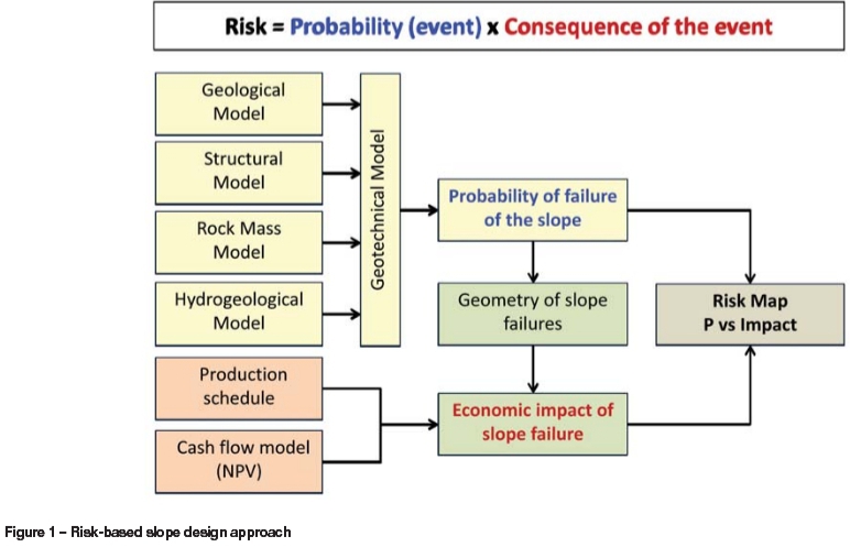
The risk analysis approach tries to solve the main drawback of the previous methodologies with regard to the selection of the appropriate acceptability criteria. Risk can be defined as the probability of occurrence of an event combined with the consequence or potential loss associated with that event:
Risk = P(event) x Consequence of the event
In the case of slopes, the P(event) is the PF of the slope and the consequences can be two-fold: personnel impact and economic impact.
The PF calculated as part of the design process is normally based on a slope stability model calculation and accounts only for part of the uncertainties of the slope. Because risk analysis sets the acceptability criteria on the consequences rather than on the likelihood of the event, a thorough evaluation of the PF of the slope is required, incorporating other sources of uncertainty not accounted for with the slope stability model. For this purpose and for the analysis of consequences of slope failure, non-formal sources of information (engineering judgment, expert knowledge) are incorporated into the process with the aid of methods such as development of logic diagrams and event tree analysis. These techniques are described in detail by Baecher and Christian (2003) with reference to geotechnical engineering problems, more commonly in the disciplines of dam and foundation engineering. However, the use of risk methods in open pit mining focuses on safety applications, based on qualitative approaches to assess operational aspects.
In the following sections, a description of the proposed risk methodology for slope design optimization is presented.
Methodology
The proposed methodology uses the framework described by the Australian Geomechanics Society (2000) with reference to the landslide risk management process, characterized by the following main steps:
➤ Identify the event generating hazards
➤ Assess the likelihood or probability of occurrence of these events
➤ Assess the impact of the hazard
➤ Combine the probability and impact to calculate the risk
➤ Compare the calculated risk with benchmark criteria to produce an assessment of risk
➤ Use the assessment of risk as an aid to decision-making.
The methodology described in this paper refers mainly to steps 2 to 5 as applied to the risk evaluation of pit slopes.
The proposed risk evaluation process for slope design is intended to quantify the impact of potential slope failures on the economic performance of open pit mines. Figure 1 illustrates the risk evaluation process and depicts the main elements of the methodology, which are described in detail in this paper. The diagram includes the main components of the conventional geotechnical slope design process as described in Stacey (2009) and incorporates the additional elements required from the mine design process.
The main objective of the methodology is the definition of the pit slope angles for mine design by applying project specific criteria to the quantified risk costs. The approach includes the following main steps:
➤ Definition of the set of slope sections for analysis covering key and critical pit areas during the mine life to provide representative cases of potential risks of slope failure within the mine plan
➤ Calculation of the probability of failure (PF) of the slopes from the analysis of stability of the selected slope sections
➤ Quantification of the economic impacts of slope failure with reference to the loss of annual profit or total project value as measured by the NPV
➤ Integration of the results of probability of failure and economic impact on an annual basis to define the economic risk map per year and for the life of mine
➤ Comparison of the risk map with criteria to assess acceptability of the design and to define risk mitigation options as required
➤ If the analysis is intended for the comparison of alternative slope design options, the process is repeated for each alternative pit layout and the results are collated in a graph of slope angle versus value and risk cost where the optimum slope angles can be defined.
A complete risk evaluation process should also include the evaluation of the safety impact of slope failures. Safety risk evaluation is discussed by Contreras et al. (2006), Terbrugge et al. (2006), Tapia et al. (2007), and Steffen et al. (2008), and is not covered in this paper.
Slope sections for analysis
The risk evaluation process requires a programme of slope stability analyses, including the critical pit areas and years in terms of potential economic impacts of eventual slope failures. This means that besides adequate information on geotechnical conditions defining the likelihood of failures, a good understanding of the mine plan is required to identify those areas and years in which the impacts of failure are likely to be greater.
The selection of the sections for stability analysis starts with the selection of the years of the mine life that represent development periods in the mine plan with similar characteristics in terms of pit geometry, production profile, and economic scenario. Figure 2 shows an example of the cumulative discounted profit of a mine plan, which is a representation of the realization of value with time. This graph facilitates the definition of the appropriate periods and representative years of mine development for the risk model analysis, which in this example corresponds to the six years defining the stepped curve.
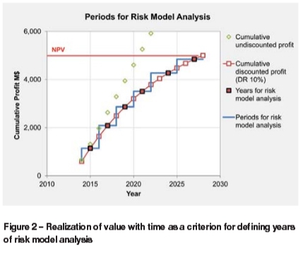
In general, probabilities of failure increase through the mine life, whereas impacts tend to maintain their levels or even decrease as mining progresses. The assumption that risk conditions of a later year (2027) represent those of early years (2025/2026) is therefore reasonable, with a minor effect on the results or (more commonly) on the conservative side. The graph in Figure 2 implies that there is a trade-off between rigour and practicality when selecting the years for analysis. Ideally, every year would have to be analysed, although this would not be practical and is probably unnecessary in the majority of cases.
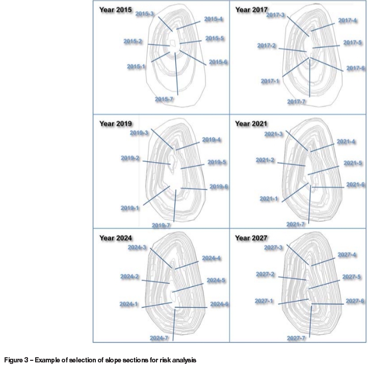
The appropriate slope sections for analysis can be selected by examination of the mine plan in the identified key years. The criterion used for this selection is based on covering the anticipated higher risk areas of the mine, which include locations where the likelihood of slope failure or the associated impact is expected to be high. Examples of the preferred locations for analysis include areas with higher or steeper slopes, sites with unfavourable geological conditions, areas with distinct characteristics such as those defined by the geotechnical domains, critical access points to mining faces, areas close to key infrastructure, and so forth. The pit development plan sketched in Figure 3 shows an example with the selection of 42 sections used in this paper to illustrate the risk process.
Slope stability analysis
The results of the slope stability analyses are reported in terms of PF values, which are calculated with the appropriate slope stability models in accordance with the relevant failure mechanisms in each domain. The methodology used for the calculation of the PF is in part determined by the type of deterministic model used for the calculation of the FS of the slope. A compilation of the methods commonly used in slope design can be found in Lorig et al. (2009). In a probabilistic stability analysis, the input parameters that represent the uncertainties are described by probability distributions. These distributions are combined within the deterministic model to define the distribution of the FS, which is used to estimate the PF of the slope. The PF is calculated as the ratio between the number of cases representing failure (FS<1) and the total number of cases of FS described by the distribution. Simple models, such as those based on the limit equilibrium method, can incorporate built-in routines to perform Monte Carlo simulations that enable the PF to be calculated relatively quickly. However, the use of more elaborate models based on stress-deformation analysis, with higher computational demands, restricts the calculation of the PF to those methods requiring a reduced number of FS entries to define its variability. Examples of such methods include those based on Taylor series expansions, the point estimate method, and the response surface methodology. Descriptions of these methods in terms of their conceptual basis are given by Baecher and Christian (2003) and Morgan and Henrion (1990). The response surface method has been used in risk-based slope design applications as described by Steffen et al. (2008). This approach has the advantage of combining the rigour of a Monte Carlo simulation with the practicality of requiring fewer FS calculations with the geotechnical model to construct the response surface used as a surrogate model in the process.
Due to practical limitations, the PF values calculated with slope models are typically the result of considering the uncertainty of the strength properties of rock masses and structures, without consideration of any other potential factors contributing to slope instability. Therefore, these PF values are incomplete representations of the likelihood of failure, and need to be adjusted as discussed later for the purpose of a risk consequence analysis.
Interpretation of probability of failure (PF) of the slope
A slope failure event could be regarded as a Bernoulli trial (also called binomial trial), which is defined as a random experiment with only two possible outcomes, success or failure, and in which the probability of success (or failure) is the same every time the experiment is conducted. According to this definition, and considering failure as the target event of analysis, if p is defined as the probability of failure, then q = (1-p) corresponds to the probability of no failure. Examples of Bernoulli trials include a 'head' after tossing a coin (p=50%, q=50%), a 'one' after rolling a dice (p=16.7%, q=83.3%) and, under certain assumptions as explained below, a failure after excavating a slope (p=PF, q=1-PF). The successive repetition of Bernoulli trials constitutes a Bernoulli process. The probability of success (or failure) is revealed in a Bernoulli process with a large number of trials. It is possible to verify that after rolling the dice a hundred times, the number of 'one' cases will be close to 17 and as more trials are considered, the better the approximation will be to the 'one in six' probability of getting a 'one'.
Strictly speaking, a Bernoulli trial refers to a discrete independent event, which is not exactly the case of the continuous process in time or space that characterizes the excavation of a pit slope. However, the consideration of the slope excavation process as a series of discrete situations, for example, excavation of consecutive slope lengths along a pit wall or annual exposure of slopes through the mine life, is a valid assumption within the framework of the risk model for slope failure, as failure events are associated with specific slope sections that are selected precisely to represent distinct conditions in terms of time of exposure and location within the pit.
The association of open pit slope failure events with a Bernoulli process enables the following interpretations based on the number of trials of the process.
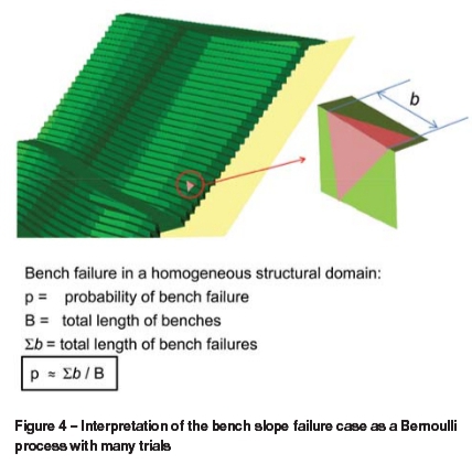
Bench slope failure in a homogeneous domain
A bench slope failure in an open pit situation could be seen as a Bernoulli process involving many trials. The probability of bench failure in a benched slope within a homogeneous structural domain corresponds approximately to the ratio between the cumulative length of failed benches and the total length of constructed benches in that domain. In this case, the entire slope could be considered as a series of consecutive realizations of a unitary slope with a length given by the typical failure width. This case is illustrated in the sketch in Figure 4 and is comparable with the situation of rolling a dice many times to verify the probability of getting a 'one'. In fact, the bench slope case can be seen as if a bench of length 'b' is constructed many times, with a percentage of those corresponding with failure situations.
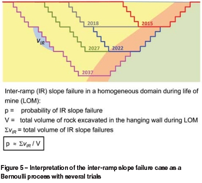
Inter-ramp slope failure in a homogeneous domain
The case of a hangingwall in an open pit mine located within a homogeneous geotechnical domain could be loosely associated with a Bernoulli process with several trials. In this case the probability of failure of the inter-ramp slopes for the life of mine could be approximated by the ratio between the cumulative volume of inter-ramp slope failures having occurred and the total volume of rock excavated during the life of mine in the hangingwall, as illustrated in Figure 5.
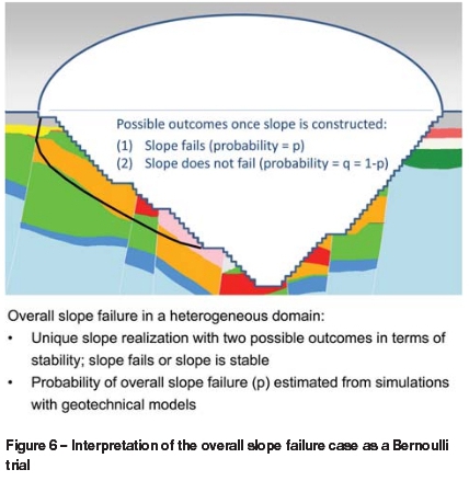
Overall slope failure in a heterogeneous domain
The case of overall slopes in open pits in heterogeneous geotechnical domains could be associated with a Bernoulli process with few trials or even with a single Bernoulli trial. The probability of failure of these slopes is not revealed in a physical manner and the estimation can be based only on simulation trials with geomechanical models representing the slopes. In this case the slope could be seen as a unique realization or trial that is not repeated in time or space, similar to the situation of a dice rolled once with two possible outcomes in terms of getting a 'one', success or failure. The overall slope failure case as a Bernoulli trial is illustrated in Figure 6.
Estimation of PF values for risk analysis
The PF values to be used in a risk evaluation process need to represent all the exposed areas of the pit in the year of analysis, and to account for all possible uncertain factors that may lead to slope failures. The PF values calculated with slope stability models refer to specific sections of the slopes and typically account only for the uncertainties associated with variability of geotechnical properties. Therefore, these limitations need to be accounted for in the set of PF values resulting from the geotechnical analysis, such that they are truly representative of the likelihood of failures in the pit areas and mine plan years of analysis. For this purpose, two types of adjustments are required to the PF values calculated with the geotechnical models: one related to the estimation of the PF of the pit wall as opposed to that of the section of analysis; and the other to the estimation of the total PF as opposed to the model PF.
Section and slope wall PF
Figure 7 shows the difference between the PF resulting from a stability analysis with a representative section of the slope and the PF value reflecting the likelihood of slope failure in a pit wall with a length greater than the expected width of the failure.
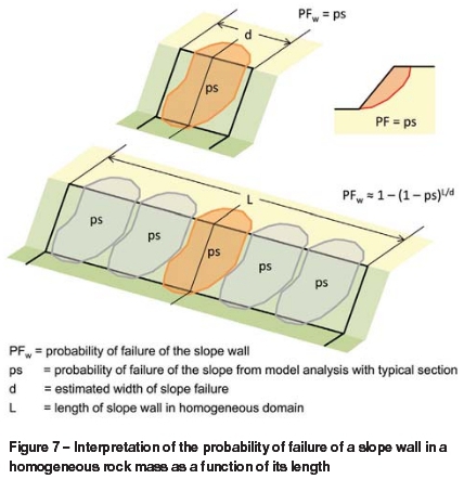
It is clear that the PF of the longer slope wall in Figure 7 is greater than that of the shorter slope shown. Considering the shorter slope as a unitary slope with a length comparable to the expected width (d) of the failure, then the longer wall with length (L) could be seen as a series of consecutive realizations of the unitary slope (Bernoulli trials). If the PF of the shorter slope is given by the probability of failure (ps) resulting from the analysis of a typical section of the slope, then the PF of the longer wall (PFw) can be estimated with the following expression:

This consideration is useful to ensure that the possibility of failure of every exposed slope in the pit is included in the risk analysis. However, the applicability of this adjustment is restricted to those situations where the assumption of homogeneity of the wall represented by the section analysed is reasonable; otherwise, the analysis of additional sections needs to be implemented.
This consideration is also important in conventional geotechnical design procedures where PF values from geotechnical analysis are compared with acceptability criteria of reference, since complying with the specified criteria on a section basis does not necessarily guarantee that the criteria are met for the slope wall.
Model and total PF
The analysis of consequences of slope failure requires that the PF of the slopes be a true reflection of the likelihood of occurrence; therefore, all possible situations leading to slope failures need to be included in the analysis. Due to practical limitations, the PF calculated with the geotechnical slope model typically accounts only for the uncertainty of the material properties, and is referred to as the model probability of failure (PFmodel) in the following discussion.
The estimation of the PF incorporating other sources of uncertainty not accounted for with slope models was discussed by Contreras et al. (2006) and by Steffen et al. (2008) using a methodology based on the analysis of source response diagrams (SRDs). The methodology is based on concepts presented by Chapman and Ward (2003) with reference to project risk management processes used in a wide range of industries. The method enabled the quantification of the contributions to the PF caused by departures from the normal conditions assumed for the design of the slopes. These variations were evaluated within various categories such as groundwater conditions, geological features, operational factors, or occurrence of seismic events. The estimated contributions were added to the PF value resulting from assuming normal conditions of design to calculate the total probability of failure (PFtotal) to be used in a risk analysis.
The methodology presented in this paper is analogous to the SRD approach described by Steffen et al. (2008), but adds some considerations regarding time in order to reflect the gradual increase, with time, of exposure to the atypical conditions evaluated. The method is appropriate for the assessment of types of uncertainties characterized by an aleatory nature. Other uncertainties not associated with frequency of events would be better treated with an expert opinion approach, with a greater reliance on experience and intuition.
There are two main types of uncertainty in geotechnical engineering - aleatory and epistemic. The former is due to the random variation of the aspect under analysis, and the latter to the lack of knowledge of the aspect. Uncertainties are quantified with probabilities, which in turn can be interpreted as frequencies in series of similar trials or as degrees of belief. Baecher and Christian (2003) provide a detailed discussion on the topic of this duality in the interpretation of uncertainty and probability in geotechnical engineering, indicating that both types of probabilities are present in risk and reliability analysis and pointing out that the separation between them is a modelling artifact rather than an immutable property of nature. Some aspects of geotechnical engineering can be treated as random entities represented by relative frequencies, and others may correspond to unique unknown events better treated as a degree of belief represented by expert opinion.
Subjectivity associated with probability estimates is a way of capturing and integrating expert judgment, only some of which may be based on hard data, and is what formal modeling of uncertainty and risk is about. Analysis, which must be based on hard data, is inherently partial and weak. The topic of subjectivity and expert opinion as a key element of risk and reliability analysis in geotechnical engineering is discussed in detail by Vick (2002) and by Baecher and Christian (2003).
The atypical conditions treated with this methodology are analysed on an annual basis, therefore each year they either occur or do not, and their annual occurrence is determined by the same underlying probability derived from a common set of conditions judged for the life of mine, either from hard data or from expert opinion or from a combination of both. These conditions suit those of a Bernoulli process and support the gradual increase of likelihood of occurrence with time estimated with the approach.
Given the probability of occurrence of a particular uncertain atypical situation leading to slope failure (Patypical) associated with a defined mine life duration in years (n), the annual probability of occurrence of this situation (patypical) can be calculated with the following expression:

The probability of failure of the slope, given that the atypical conditions occur (PFmodel |atypical), could be evaluated with the slope stability model. The results of such analysis could be expressed as a factor (fatypical) of the model probability of failure evaluated under normal conditions. This factor could be the result of sensitivity analysis where different scenarios of the atypical condition are evaluated. Therefore:

Finally, the probability of failure of the slope due to atypical conditions (PFatypical) can be calculated for a particular year (i) of the mine plan as follows:

The probability of failure of the slope due to atypical conditions (PFatypical) is added to the model probability of failure (PFmodel) from the geotechnical analysis under normal conditions of design to define the total probability of failure (PFtotal) appropriate for the risk evaluation process. The addition of the probability values is carried out with the following generic expression, which is based on the concept of system reliability:

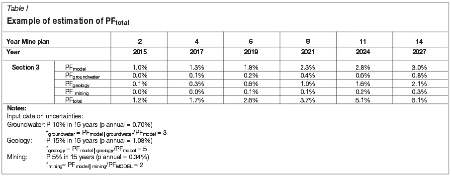
The method of calculation of PFtotalfrom PFmodelis illustrated with an example where the contributions from uncertainties related to groundwater, geology, and mining are added to the PF calculated with the geotechnical model for the slope represented by Section 3 of the mine case shown in Figure 3. Equation [5] can be extended to account for these three aspects as follows:
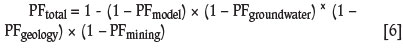
The results of this analysis are indicated in Table I and Figure 8, and the input probabilities and factors are indicated in the footnotes to the table. Equations [2], [3], and [4] are used to calculate the terms in Equation [6]. The calculated contributions of each uncertain aspect to the PFtotal are shown by the curves in Figure 8.
The uncertainties considered in the example of Table I and Figure 8 are intended to present the concept of adding uncertainties of random character not included in the geotechnical models for slope analysis. However, the relevant uncertainties not included in the models need to be identified and assessed on a project-specific basis. It may be that factors such as unknown stress conditions, actual pit geometry variations, or other specific situations are the more relevant aspects that would contribute to the overall PF in a given project. Also, the best way to treat a particular uncertainty needs to be defined based on its prevalent nature (i.e. aleatory or epistemic).
In the slope stability evaluation process, the consideration of the potential effect of atypical situations leading to failure means that no matter how stable a slope might appear in terms of the calculated stability indicators, the probability of failure for the risk analysis is never zero and therefore the risk of failure is always present.
Model uncertainty
Model uncertainty in the slope stability analysis can be evaluated through the critical FS value (FScritical) used to define failure with the model. This type of uncertainty arises through systematic biases in input parameter determinations and idealizations in the calculation process, leading to the result that failure occurs for some FScritical value that may not be unity, as commonly assumed. Bias in parameter determination is inevitable, and is handled by calibration to slope performance. Model idealizations arise from simplifications required to represent the geometry, material behaviour, etc. Some aspects of model idealizations will tend to reduce FScritical, while others might raise FScritical. The effect of the parameter bias and model uncertainty is to produce an uncertainty band that is centred on the underlying bias. An evaluation of FScritical based on the comparison of actuarial failure rates versus nominal factor of safety was carried out for the risk study of the Chuquicamata pit as described by Tapia et al. (2009). Unfortunately, this approach requires local historic records, which are not always available; therefore, judgement as well as reference to similar projects is the only practical option left to account for this uncertainty.
Estimation of economic impact of slope failure events
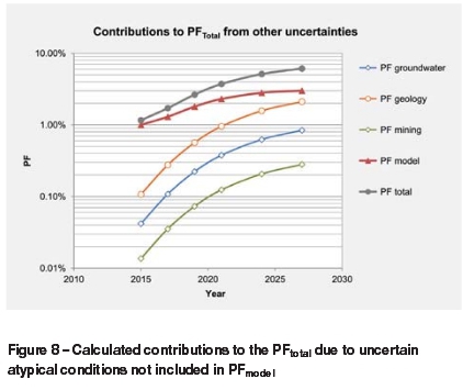
The economic impact of a slope failure can be measured through the quantification of the effect of this event on the value of the mine plan as measured by the NPV. The NPV corresponds to the cumulative discounted annual profits during the life of the mine and is normally defined as the result of a mining scheduling and optimization process carried out with specialized software. In general, the economic impact of a slope failure is a result of the disruption of the planned ore feed during the time required to restore the site, and the additional costs caused by these activities. Figure 9 illustrates the conceptual basis for the estimation of impacts of slope failures. The economic impact of a slope failure is defined as the difference between the NPV of reference (mine plan without failures) and the re-calculated NPV incorporating the effects of the failure on production and cost components.
Production may be disrupted by different factors such as interrupted access to the mining faces, covered ore, variations of grade when alternative sources of ore are used to mitigate the effects of the failure, and so forth. The additional costs are caused by the additional material handling and rescheduling of equipment required to restore the site affected by the failure.
A simplified approach to quantifying the impact of a failure consists of calculating the differential NPV due to the failure, using a cash flow model that includes the estimated effects of the failure on production and costs. The impact on production is simulated by means of a reduction factor of the mined tons, which is estimated by considering aspects such as the magnitude, location, and time of occurrence of the failure and the flexibility of the mine plan to provide alternative ore feed sources. Engineering judgment and supporting reference data are normally used to estimate the impact factors from each failure event.
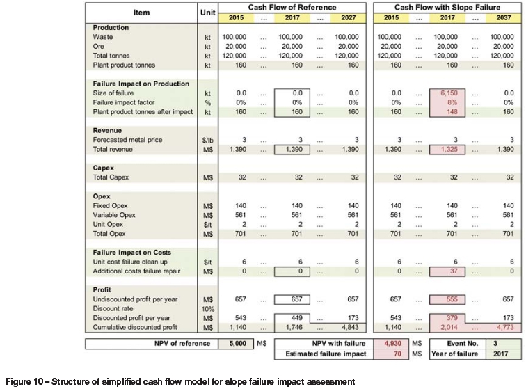
The simplified cash flow model should include production data per mining phase, revenue calculations, as well as operating and capital costs, and needs to be calibrated against the reference NPV in the mine plan. An example of the structure of the simplified cash flow model used for the calculation of economic impact of slope failures is shown in Figure 10. The example illustrated shows that the impact on production affects the plant product tons and the revenue, which, together with the additional costs of restoring the site, ultimately reduces the net benefit and consequently the NPV.
One drawback of the simplified approach is that the complex effect of variations of the planned grade feed when drawing from stockpiles cannot be simulated accurately. For this reason, the calculated impacts need to be validated with results derived from a thorough evaluation of selected key events in a similar manner as they would be evaluated in a real-life situation, where specific re-designs of the plan would be carried out to minimize the impact of the slope failure.
Risk map for economic impact analysis of slope failure
The results of probability of failure and economic impact calculations for individual failure events are used to construct the economic risk map per year and for the mine life. The risk map defines the relationship between the probability of a particular economic impact and the magnitude of that impact; and accounts for different situations of occurrence of events in a year, including isolated occurrences, concurrent occurrences of the different possible combinations of the events, and no occurrence of any event.
The risk map construction process is based on the concept of event tree analysis. The event tree is a diagram that connects a starting event with the ultimate consequence under evaluation through a series of intermediate events based on a cause-effect relation. The events are quantified in terms of their likelihood of occurrence, thus enabling the assessment of the final outcomes in terms of their probabilities of occurrence. The event tree methodology for economic impact, originally described by Tapia et al. (2007) with reference to the case of the Chuquicamata mine and later discussed by Steffen et al. (2008) and in Wesseloo and Read (2009), relies on subjective inputs of probability for the events in the tree to produce an assessment of the expected likelihood of three categories of economic impact (force majeure, loss of profit, and minor impact). The main drawbacks of this methodology are that there is no consideration of the possible occurrence of various events in a year and that the impacts are assessed only in terms of likelihood, without a clear definition of the magnitude of these impacts.
The combined analysis of probability and economic impacts with event trees is discussed in detail by Baecher and Christian (2003), including examples of consequence analysis where the probabilities of events and the respective impacts in monetary terms are multiplied to produce risk cost values used as a measure of the risks. One drawback of this approach is that the outcomes of the analysis do not represent actual possible impacts, but rather amounts weighted by the respective probabilities. This characteristic of the risk calculation is referred to by Baecher and Chirstian (2003) as 'risk neutrality', where high-probability low-consequence outcomes are treated as equivalent to low-probability high-consequence outcomes, as long as the product is the same. The reality is that the events either do or do not occur and consequently the impacts will either be caused or not - intermediate results are not possible.
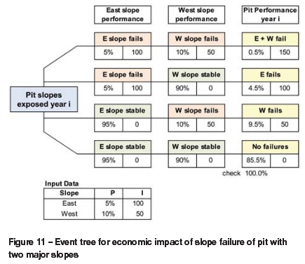
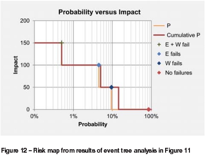
The proposed risk evaluation approach is carried out with a separate accounting for probabilities and impacts and the end results from the event tree branches are used to construct the risk map. The method is illustrated in Figure 11 for the simple case of a pit with two major slopes named East and West, with PF values of 5% and 10% and impacts of 100 and 50, respectively. The sum of the probabilities of the four possible outcomes depicted with the tree is 100%, indicating that all the possible combinations of events have been adequately accounted. The risk map constructed with the results of the event tree is shown in Figure 12. The cumulative probability curve of particular impacts constitutes the economic risk envelope of the pit.
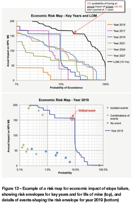
The risk map of a more realistic case, such as the mine plan described in Figures 2 and 3, is constructed for the individual key years selected to represent the various periods of the mine plan, which are then used to define the overall risk map for the life of mine, as shown in Figure 13. The graph at the top shows the various risk envelopes and the graph at the bottom shows the details of the failure events of year 2019 used to construct the envelope. The risk envelopes are cumulative probability distributions of impacts and are interpreted as indicated in the graph at the top of Figure 13 for the case of impacts with a 10% probability of exceedance. The result for the indicated case would be a 20% probability of having an annual impact of at least $160 million over a period of 15 years. The display of the individual events in the risk chart is useful to identify critical events causing an increase of the risk level as measured by the envelope, as depicted in the example shown on the graph at the bottom of Figure 13.
Probability concepts for construction of risk map
The slope failure events considered for the construction of risk maps correspond to large-scale failures and are analysed on a year-by-year basis. The events are treated as Bernoulli trials and are characterized by a probability of occurrence (p) given by the calculated probability of failure of the slope (PF) and the respective impact (i) estimated in monetary terms. The risk map construction is based on the calculation of the probability (P) of having an economic impact (I) considering different possible situations of occurrence of the events as explained below.
In the following expressions, the terms with sub-indices i, j, and k (in bold) represent the occurring events, and those with sub-indices r, s, and t (in italic), refer to the non-occurring events:
➤ Occurrence of single events:
Pi = pi x (1 - pr) x ... x (1 - pt)
Ii = ii
➤ Multiple occurrence of events:
Pi...k = pi x... x pk x (1 - pr) x ... x (1 - pt)
Ii...k = ii + ... + ik
➤ A particular case of the multiple occurrence described in (2) is the occurrence of all the events in a year:
Pi...k = pi x pj x ... x pk
Ii...k = ii+ ij+...+ ik
➤ No occurrence of any of the events:
Pr...k= (1 - pr) x (1 - ps) x ... x (1 - pt)
Ir...t = 0
The total number of possible cases of occurrence of events (T) for (n) independent events in a year effectively corresponds to the number of branches of the respective event tree, and is given by the following expression:

From this number, n cases correspond with the occurrence of isolated events and one case to the non-occurrence of any of the events. The remaining N cases correspond with the occurrence of combinations of two or more events. The generic expression to calculate the number of combinations (N) of 2 or more events that can be obtained with ( n) events is:
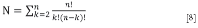
or

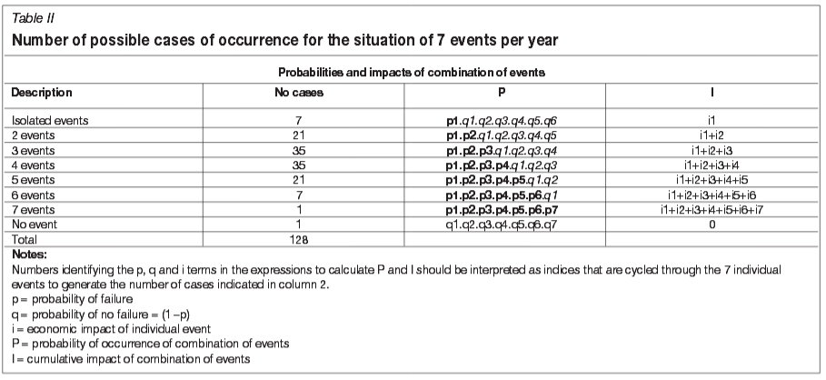
The calculation of all possible probability and impact pairs can be done without constructing the respective event tree, which would be a cumbersome task as the number of branches of the tree increases exponentially with the number of annual events. A summary of the probabilities and impacts of the different possible combinations of 7 events per year is presented in Table II. In this table, p corresponds with the probability of occurrence (failure) and q with the probability of no occurrence (no failure) of the respective events. The number of cases in Table II is calculated with Equation [8] and the total number of possible occurrences of the 7 events is 128. This is the number of data points available to construct the risk map as described in the following section.
Construction of the risk map
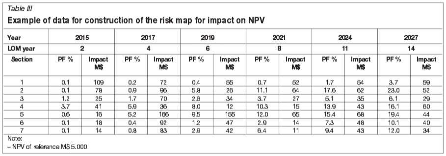
An example of the input data required for the construction of the risk map is presented in Table III. The data includes the probability of slope failure and the associated impact of seven sections per year and six years of analysis, on the mine plan of 15 years' duration, as described in Figures 2 and 3. The PF values in Table III are based on the results of the geotechnical analysis of the respective sections and cater for the atypical conditions leading to failure discussed previously.
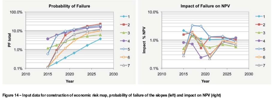
The data in Table III is shown in graphic form in Figure 14 to illustrate the variations of the probability of failure and associated impacts with pit development. The graph at the left of Figure 14 is consistent with the increasing likelihood of failure of the slopes expected as the pit grows deeper. The curves in the graph at the right of Figure 14 do not show a unique trend in the variation of impact with pit growth, as impacts are dependent on the particular characteristics of ore exposure and ore access during the development of the mining phases.
The risk map construction is carried out per year and the data is used to calculate the pairs of values of probability and impact associated with all possible combinations of failure events using the expressions in Table II. The 128 data pairs for each year of analysis are sorted and used to construct the respective probability distribution graphs of impacts. These graphs include a frequency distribution histogram and the corresponding cumulative frequency curve as shown in the graph at the top of Figure 15 for the year 2019 of the example in Table III.
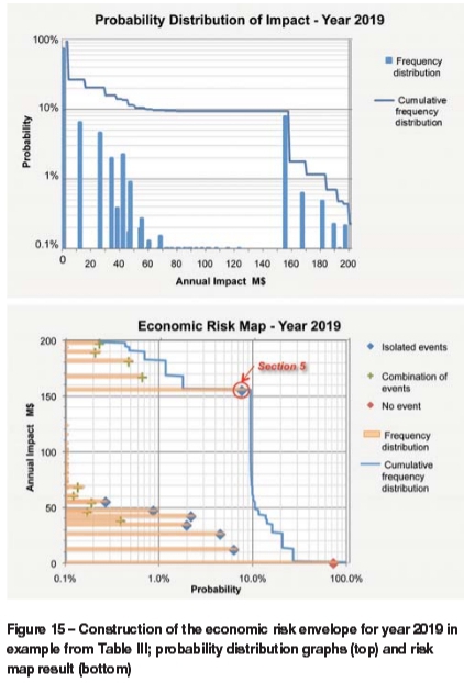
The risk map result is shown in the graph at the bottom of Figure 15. The graph contains the probability distribution plots with the axes swapped to conform with the typical way in which risk acceptability criteria is presented, as discussed in the following section. The graph also includes the data points representing the various possible occurrences of the events. The blue data points correspond with isolated events, the green points with the concurrent occurrence of combinations of events, and the red point on the horizontal axis represents the particular situation of no occurrence of any of the events. Not all the data points are visible because many of them correspond with low probability values outside the range of the logarithmic scale used in the graph.
Nevertheless, these low-probability events have an influence on the final result, which is captured by the cumulative distribution curve. Typically the risk map excludes the frequency distribution histogram in order to avoid an overcrowded graph. A practical way of defining the cumulative distribution curve of impacts is through a Monte Carlo simulation where the seven failure events are modelled with Bernoulli distributions (also called yes-no distributions) and the impacts calculated accordingly.
The probability values given by the risk envelope should be interpreted as probabilities of exceedance of the respective value, as this curve corresponds to a cumulative probability distribution associated with all possible combinations of events considered. The risk envelope defines the economic risk profile for the respective year. The analysis of the patterns shown by the data points representing the occurrence of individual events is valuable for identifying critical events that push the risk envelope towards the upper right side of the graph. One example of such an event would be the slope failure associated with Section 5 in year 2019 as shown in Figure 15.
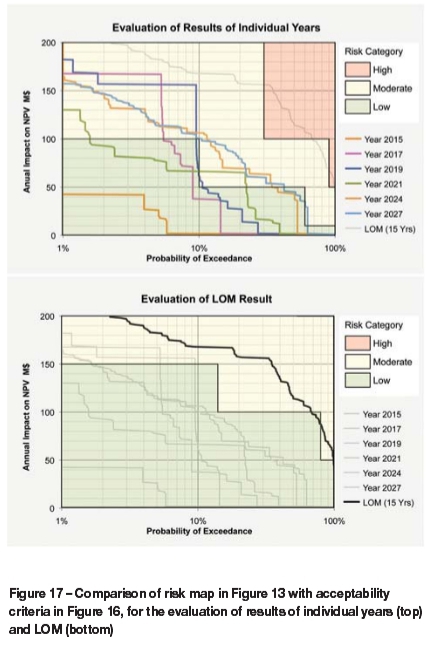
The risk envelopes of the six representative years included in Table III were used to construct the economic risk map for the life of mine as shown in the graph at the top of Figure 13. The procedure is based on compounding the probabilities of the various years for fixed values of impact, considering the periods of the mine life represented by each year as shown in Figure 2. The probability values are added using the concept of reliability of a system. In this particular example the probability of an economic impact for the life of mine (PLOM) for a given impact is calculated from the corresponding annual probabilities using the following expression:
The exponents in this equation correspond to the number of years represented by the probability value in the respective term. The sum of these exponents is 15 and corresponds with the total number of years of the mine plan.
A different perspective of the economic risk could be provided by the analysis of impacts on annual profits, because in this way, future amounts are not discounted to present values, which in some cases causes a perceived distortion of value. Risk maps based on the impacts on annual profits can be calculated following a similar process to that described for impacts on NPV. Furthermore, the analysis can be carried out with impacts measured in terms of commodity product rather than monetary units, in order to avoid possible distortions caused by the assumptions on commodity prices.
Uses of the risk map
There are two main uses of the risk map described in this paper; one is for the evaluation of a specific open pit design in terms of economic risk by comparing the result with acceptability criteria, and the second refers to the comparative analysis of open pit design options, in terms of value and risk, to identify optimum pit layouts.
Comparison with acceptability criteria
The risk map can be used to assess a specific pit design by comparing this result with acceptability criteria specifically defined for the project. The result of this analysis enables the identification of the more appropriate risk treatment strategies to advance the project. In particular, the comparison with acceptability criteria is useful for the identification of those years of more relevance in terms of potential economic impacts and the respective critical pit areas causing those risks. This information is valuable for the definition of the areas requiring more investigation in further stages of study and for the evaluation of mitigation strategies to reduce the risks.
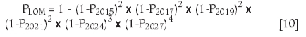
Risk acceptability criteria are normally described in the form of a matrix in which risk is categorized in terms of likelihood of occurrence along the horizontal axis and severity of the impact up the vertical axis, to define high (H), medium (M), and low (L) risk levels. This type of matrix was originally developed for use in qualitative methods of risk analysis, with the scales adapted or adjusted to suit different types of application (Joy and Griffiths, 2005). However, a more precise definition of the scales of likelihood and severity results in acceptability matrices especially suited for the use in quantitative risk evaluation methods such as that based on the risk map construction described in this paper. An example of a risk acceptability matrix is shown in Figure 16, where likelihood and impact categories are defined specifically for the project setting at hand. The risk matrix also provides guidelines for risk treatment actions to follow, based on the risk results.
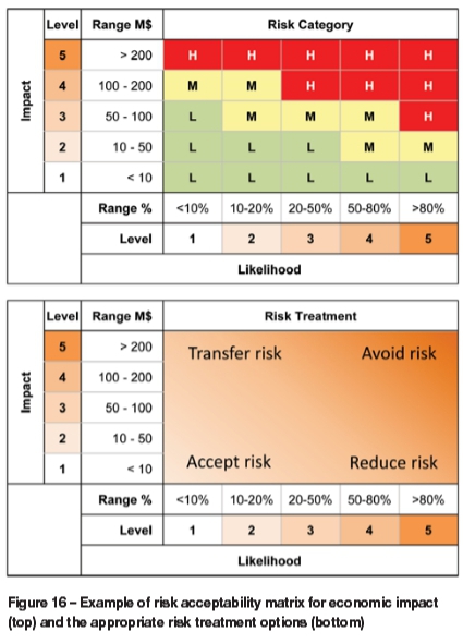
The use of the risk acceptability matrix in Figure 16 is illustrated in Figure 17, where the risk map results shown in Figure 13 are compared with the acceptability criteria. The criteria presented in Figure 16 are intended to adjudicate risk envelopes of individual years and need to be converted to the appropriate values for the analysis of the LOM envelope. The conversion is carried out with the same approach used to calculate the LOM envelope from the annual curves. This involves adding the annual probabilities using the concept of system reliability, considering a 15-year time span.
In the example presented in Figure 17 the grey curves are included for reference but are not intended to be compared with the displayed risk zone categories. The evaluation of the individual years (top graph) indicates a low to moderate risk profile for all years, with the envelope of year 2019 showing a local elevated risk associated with conditions of Section 5, as depicted in Figure 15. This finding constitutes a pit optimization opportunity and illustrates the way in which the risk envelopes can be used to identify areas requiring attention in further stages of study. The evaluation of the LOM risk envelope illustrated in the graph at the bottom of Figure 17 suggests a moderate risk level of the overall mine plan.
Value and risk analysis of design options
The risk map can also be used to define risk cost values of alternative pit slope design options that need to be compared in terms of economic risk performance. Risk cost values are used to construct the value and risk profile for changing slope geometries, which provides the elements for screening of options in an early design stage and facilitates the identification of the main features of pit geometry for an optimum design.
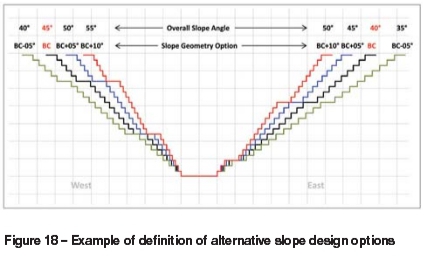
Generally, a base case pit slope design is available, which is the result of conventional slope design methods based on FS or PF criteria, or local experience in terms of slope performance in particular geological settings. The base case mine plan typically corresponds with a balanced risk condition, therefore slope design options on both sides of the base case are required to define the relationship between the slope angle and the value and risk condition of the pit layout. An example of the construction of alternative pit slope geometries for the risk analysis from the base case layout is illustrated in Figure 18. In this case the alternative slope designs are generated by flattening the base case by 5° and steepening by 5° and 10°, resulting in nominal slope design angles of 35°, 40°, 45°, and 50° for the east wall and 40°, 45°, 50°, and 55° for the west wall.
The risk maps for the four alternative pit design options are constructed using the respective slope stability results and economic impact assessment of slope failures. An example of the risk envelopes for the life of mine of the four slope design options shown in Figure 18 is presented in Figure 19. The risk envelopes are compared with the acceptability criteria (Figure 16), adjusted for a life of mine of 15 years. The graph also includes the risk cost values read from the envelopes for probabilities of exceedance of 10%, 50%, and 90%, which are used to assess the options in terms of value and risk.
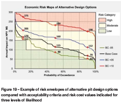
The risk envelopes in Figure 19 indicate that the base case -05° (BC-05) is in the low to moderate risk threshold, the base case (BC) and base case +05° (BC +05) are in the moderate risk area, and the base case +10° (BC+10) option falls in the high risk area. The comparison with the acceptability criteria does not provide sufficient elements to establish a clear contrast between the options in terms of their risk performance.
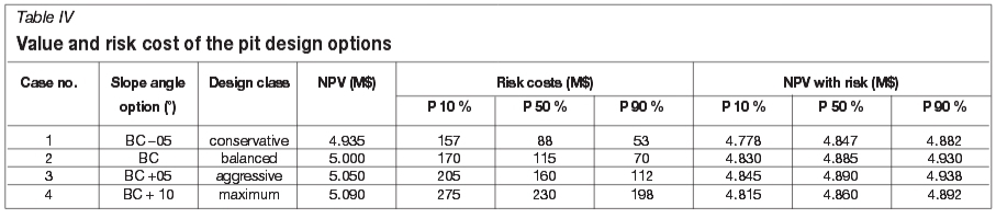
The risk cost values indicated in Figure 19 are used to construct the value and risk profiles of the slope design as shown in Table IV and Figure 20. These results show the variation of value in terms of NPV and risk cost for the various slope design angles. The design options have been categorized in terms of the risk results as conservative, balanced, aggressive, and maximum, for the slope design cases of BC -05, BC, BC +05, and BC +10, respectively. The risk cost or costs of impact of slope failures have an inverse relationship with the probability of incurring those costs, with higher probabilities of small impacts and lower probabilities associated with large impacts.
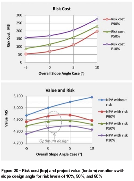
The graph at the top of Figure 20 shows the typical increase of risk cost with increasing slope angle for various levels of likelihood of impacts. The risk cost values were used to construct the NPV with risk curves shown in the graph at the bottom of Figure 20. This graph shows a steady increase in NPV with increasing slope angle when no risk aspects are considered. However, once the risk cost is included in the analysis, the curve of value shows an inflexion point as the slope steepens, defining the angle that represents the optimum balance between value and risk. The results in Figure 20 would serve to confirm the adequacy of the base case design, and would suggest a possible optimization opportunity by steepening the slopes by up to 3 degrees.
Information such as that included in Figure 20 constitutes a valuable tool to optimize the pit design and to bracket the overall slope angles for further phases of study.
Conclusions
The methodology presented provides a rational approach to defining, at an early stage of a mine, the main features of pit geometry reflecting the appropriate balance between value and risk, in accordance with the specific conditions of the project. The process considers both the likelihood of occurrence of individual slope failure events and the resulting economic impacts from all possible combinations of occurrence of these events on an annual basis and for the mine life. The economic risk map constructed for a particular pit slope layout can be used in an optimization process by comparing this result with project-specific acceptability criteria. When the process is used for the evaluation of alternative design options, the risk maps can be used to make risk cost estimations to calculate the variation of project value with slope angle. These results enable the definition of the main features of pit geometry reflecting the appropriate balance between value and risk, in accordance with the specific conditions of the mine, which allows the rationalization of requirements of geotechnical information at different stages of project development, once risk criteria have been defined.
References
Australian Geomechanics Society. 2000. Landslide risk management concepts and guidelines. AGS Sub-Committee on Landslide Risk Management, Sydney, Australia. [ Links ]
Baecher, G.B., and Christian, J.T. 2003. Reliability and Statistics in Geotechnical Engineering. Wiley, Chichester, UK. [ Links ]
Chapman, C. and Ward, S. 2003. Project Risk Management: Processes, Techniques and Insights. 2nd edn. Wiley, Chichester, UK. pp. 148-150. [ Links ]
Contreras, L.F., Lesueur, R., and Maran, J. 2006. A case study of risk evaluation at Cerrejon Mine. Proceedings of the International Symposium on Stability of Rock Slopes in Open Pit Mining and Civil Engineering Situations, Cape Town, South Africa, 3-6 April 2006. Symposium Series S44. Southern African Institute of Mining and Metallurgy, Johannesburg. [ Links ]
Contreras, Lf. and Steffen, O.K.H. 2012. An economic risk-based methodology for pit slope design. Newsletter of the Australian Centre for Geomechanics (ACG), vol. 39, December 2012. [ Links ]
Harr, M.E. 1996. Reliability-based Design in Civil Engineering. Dover Publications, Mineola, New York. [ Links ]
Joy, J. and Griffiths, D. 2005. National Minerals Industry Safety and Health Risk Assessment Guideline. Minerals Council of Australia. Version 4, Jan. 2005. [ Links ]
Lorig, L., Stacey, P., and Read, J. 2009. Slope design methods. Guidelines for Open Pit Slope Design. Read, J. and Stacey, P. (eds). CSIRO Publishing, Collingwood, Victoria. pp. 237-264. [ Links ]
Morgan, M.G. and Henrion, M. 1990. Uncertainty: a Guide to Dealing with Uncertainty in Quantitative Risk and Policy Analysis. Cambridge University Press. [ Links ]
Read, J. 2009. Data Uncertainty. Guidelinesfor Open Pit Slope Design, Read, J. and Stacey, P. (eds). CSIRO Publishing, Collingwood, Victoria. pp. 214-220. [ Links ]
Ross, S. 2010. A First Course in Probability. 8th edn. Pearson Prentice Hall, New Jersey. [ Links ]
Sjoberg, J. 1999. Analysis of large scale rock slopes. Doctoral thesis, Division of Rock Mechanics, Lulea University of Technology, Lulea, Sweden. [ Links ]
Stacey, P. 2009. Fundamentals of slope design. Guidelinesfor Open Pit Slope Design. Read, J. and Stacey, P. (eds). CSIRO Publishing, Collingwood, Victoria. pp. 1-14. [ Links ]
Steffen, O.K.H. 1997. Planning of open pit mines on a risk basis. Journal of the Southern African Institute of Mining and Metallurgy, vol 97, no. 1. pp. 47-56. [ Links ]
Terbrugge, P.J., Wesseloo, J., and Venter, J. 2006. A risk consequence approach to open pit slope design. Journal of the South African Institute of Mining and Metallurgy, vol. 106, no. 7. pp. 503-511. [ Links ]
Steffen, O.K.H., Contreras, L.F., Terbrugge, P.J. and Venter, J. 2008. A risk evaluation approach for pit slope design. Proceedings of the 42nd US Rock Mechanics Symposium, 2nd US-Canada Rock Mechanics Symposium, ARMA, San Francisco, USA, June 30 - July 2, 2008. [ Links ]
Tapia, A., Contreras, L.F., Jefferies, M., and Steffen, O.K.H. 2007. Risk evaluation of slope failure at the Chuquicamata Mine. Proceedings of the 2007 International Symposium on Rock Slope Stability in Open Pit Mining and Civil Engineering, Perth, Australia, 12-14 September 2007. Potvin, Y. (ed.). Australian Centre for Geomechanics. [ Links ]
Vick, S.G. 2002. Degrees of Belief: Subjective Probability and Engineering Judgment. American Society of Civil Engineers, Reston, Virginia. [ Links ]
Wesseloo, J. and Read, J. 2009. Acceptance criteria. Guidelinesfor Open Pit Slope Design. Read, J. and Stacey, P. (eds). CSIRO Publishing, Collingwood, Victoria. pp. 221-236. [ Links ]
Received Jul. 2014
Revised paper received Jan. 2015
1 In non-technical literature, 'likelihood' is usually a synonymfor 'probability', but in statistical usage, a clear technical distinction is made. Here, probability offailure refers to the estimatedfrequency of FS<1 cases with the model assuming that this conditions representsfailure. PF can take values only between 0 and 1. The likelihood offailure is a quantity not constrained and refers to the chances of actualfailure, given the results of the stability analysis.

