GENERAL PAPERS

 

Stochastic simulation for budget prediction for large surface mines in the South African mining industry

 

 

J. Hager; V.S.S. Yadavalli; R. Webber-Youngman

University of Pretoria, South Africa

 

 

---

SYNOPSIS

This article investigates the complex problem of a budgeting process for a large mining operation. Strict adherence to budget infers that financial results align with goals. In reality, the budget is not a predetermined entity but emerges as the sum of the enterprise's operational plans. These are highly interdependent, being influenced by unforeseeable events and operational decision-making.
Limitations of stochastic simulations, normally applied in the project environment but not in budgeting, are examined and a model enabling their application is proposed. A better understanding of budget failure in large mines emerges, showing that the budget should be viewed as a probability distribution rather than a single deterministic value.
The strength of the model application lies with the combining of stochastic simulation, probability theory, financial budgeting, and practical scheduling to predict budget achievement, reflected as a probability distribution. The principal finding is the interpretation of the risk associated with, and constraints pertaining to, the budget.
The model utilizes a four-dimensional (space and time) schedule, linking key drivers through activity-based costing to the budget. It offers a highly expressive account of deduction regarding fund application for budget achievement, emphasizing that 'it is better to be approximately right than precisely wrong'.

Keywords: probabilistic logic, Monte Carlo, simulation, NPV, budget

---

 

 

Introduction

One of the biggest questions confronting senior management of a mine, regardless of its size or mining methodology, is: 'Why does the budget of a mine become so far removed from reality that it ends up being useless?'

The extraction of minerals is an expensive endeavour, with budgets often amounting to billions of rands, and unlike a manufacturing process, is based on a resource that is depleting with each production year. There are also factors unique to mining that make the environment challenging, including the extreme volatility of commodity markets and surety of the mineral reserves. The usual approach to dealing with these challenges is to use a rigorous budgeting process.

The budget is the single most important document that regulates the production of a mine. All the strategies, tactics, and plans are ultimately based on attaining the targets set in the budget. Investors and executive managers of resource companies judge performance and make decisions primarily based on the budgets of the mines. The budget, however, is expressed in exact amounts, which obscure (or ignore) the variability of the mining environment.

Deviations from the budget are often waived as uncontrollable elements or force majeure such as more rain than expected, unfavourable exchange rates, or strikes. Revisions to the underlying inputs (physical standards) that drive the budget are sometimes considered, but then such physical standards are also stated as exact values, ignoring their inherent variability. Random and seasonal fluctuations are aggregated into single values and treated as deterministic. Interdependability and accompanying (common-mode) risk is neglected. The result is that the budget does not have a fair chance of accurately forecasting reality.

The budgeting process for a large mine is especially complicated and arduous, needing detailed inputs from every department over a six-month period before it is finally compiled. Although management does measure the budget carefully, its action is only retrospective - i.e. the fact is known only after the budget has failed (either negative or positive) - and the autopsy then turns into finding a scapegoat. Decisions about the application of scarce capital sometimes appear to be somewhat arbitrary. There is no decision-making methodology established that dictates where funds applied (spent) will have the greatest impact on the budget.

The importance of increasing the confidence in achieving the budget, while simultaneously giving the assurance that the budget is accurate and 'strict' enough, cannot be over-emphasized. This article proposes a methodology that addresses the lack of budgeting accuracy by addressing the inherent uncertainty in a mining operation.

 

Methodology

To achieve the necessary budget accuracy, a detailed modelling tool is required. The model should be able to replicate the actual mining both in time and actual spatial translation - i.e. travelling distances and specific physical attributes must be coupled to the mine layout and assets utilized, taking cognisance of the particular equipment fleet and uniqueness of the beneficiation process, as well as the specific geological factors that govern the resource. The model should be able to replicate the budget from first principles to within 1% accuracy.

Once the detailed tool is in place and calibrated, the key operational performance drivers of the budget are determined. These are the drivers that have the most influence on the budget, and also have the largest variance. The main concept is that if two or more key drivers (that have a large impact) have large variances (as opposed to their budget assumptions) and are interdependent of each other, the probabilities of each can be multiplied to give a new probability. This new probability will have a larger 'spread' than either of the individual drivers. This leads to instability in terms of budget achievement.

The problem with the above is that if too many drivers with too large a spread are chosen, the resultant probability will be unrealistic and unusable, i.e. multiplication of a lot of fractions quickly approaches zero (this is in all probability the main reason why stochastic simulation is unsuccessful in the budget process and is therefore never applied). It is therefore clear that the key drivers must be carefully selected. These drivers should be compiled from different secondary probabilities that can be influenced (or manipulated) to optimize the distribution of the primary probability.

This leads to the investigation of how these first-order (prime) probabilities can be influenced or manipulated to increase confidence, so the budget can be achieved. The logical deduction is that it will be mostly through the application of money, i.e. to fix something, buy more, pay someone to do it, etc. This culminates in the final objective, to provide a realistic budget, expressed as a probability distribution, and show where scarce capital should be applied to achieve the optimum return.

The basic assumption is that all parameters that can influence the budget will conform to some type of probability distribution. The following distributions were considered: triangular, normal, and Weibull. These will be sufficient to describe any deviation. Due to the ability of a three-parameter Weibull distribution to closely approximate a normal distribution, the normal distribution was ignored.

Probabilistic logic and 'stochasticity'

The basic aim of probabilistic logic is to make use of probability theory in combination with logic. Probability theory is used to handle uncertainty, while deductive logic is used to exploit structure. One of the problems with probabilistic logic is that it tends to multiply the computational complexities of the probabilistic and logical components, resulting in an answer that is too vague to have practical meaning. Josang (2009) remarks that probabilistic logic by itself finds it impossible to express input arguments with degrees of ignorance as, for examples, reflected by the expression 'I don't know'. The generally accepted practice, to provide values without supporting evidence, will generally lead to unreliable conclusions, often described as the 'garbage in - garbage out' syndrome.

Risk and uncertainty

Risk (and the chance of loss), i.e. in the event that the situation can lead to both favourable and unfavourable outcomes, is the probability that the event outcome will be unfavourable, i.e. an unwanted event, while uncertainty is the indefiniteness associated with the event, i.e. the distribution of all the possible outcomes. Uncertainty is an intangible value (Elkjaer, 2000).

The main problem with the budget is that it uses only point estimates. Discrete estimates by themselves, are insufficient for good decisions (US Air Force, 2007) or a good budget.

The underlying probability distributions inherent to the production process will influence the outcome, for example no two trucks travel at exactly the same speed - and no two shifts produce exactly the same saleable product. It is therefore obvious that the answer to achieving the budget lies in the uncertainty of these cornerstones of production, which must be understood so that the probability of success may be improved (or positively influenced).

It is clear that the single deterministic point value for a budget is a fallacy, since the chance of achieving it exactly in a highly complex environment is zero. As SAP^® is widely used in large mining environments, Table 600, which is a summary of the main cost buckets of the budget, was analysed as a first step. This was further distilled by using a standard Pareto analysis to determine the most important cost buckets. A Monte Carlo simulation was then used to give the distribution of outcomes. (This simulation failed, as is explained below). From the literature it is clear that Monte Carlo simulation is used mainly for capital budgeting of large projects (Clark, 2010). Such simulations are concerned with the cost of the project, while this model concentrates on the uncertainty inherent in the production process and regards cost fluctuations as risk i.e. uncontrollable (but explainable), for example, price increases in diesel, electricity, etc.

The cost buckets were then combined to describe the cost function, broken down into fixed and variable cost. Income (through product sales) was added to allow the results to be expressed as a net profit (prior to tax and cost of capital). The probability distributions were assumed to be triangular with a lowest, highest, and most probable value (US Air Force, 2007). This methodology did not work, since the multiplication of uncertainty leads to a wider spread of probabilities - to the extent that it is clearly an irrational approach and most probably is the reason why Monte Carlo simulation is not used in the standard budgeting process.

A different approach was indicated, and the drum-buffer-rope (DBR) production planning methodology from the theory of constraints (TOC), as originally proposed by Eliyahu M. Goldratt in the 1980s, was considered. Schragenheim and Dettmer (2000) summarize the drum-buffer-rope as striving to achieve the following:

➤ Very reliable due-date performance

➤ Effective exploitation of the constraint

➤ As short a response time as possible, within the limitations imposed by the constraints.

The problem with the DBR methodology is that althoughthe beneficiation plants (specifically the tipping bins of these plants) are normally defined (through TOC) as the bottleneck, the analogy is not a true one as the mining process differs from the manufacturing production process. It should rather be described as a trail run with a specific obstacle that all the runners have to cross. It is clear that if trucks are seen as a buffer, the logical response would be to over-truck the constraint. However, in the analogy of trail running, this is the worst possible decision. More athletes trying to cross the same obstacle at the same time results in more interference with each other and a slower throughput.

Envision athletes on a trail run. Some run faster and some slower. Some stumble and block others. There is no rope (communication once the athletes are running), and this is exactly the problem with production haul trucks. Breakdowns, bad road conditions or secondary work on the road, intersections etc. cause unpredictable delays that can be handled only by stochastic methods.

The logical solution is to express the budget as a probability distribution through examining the effect of the inputs in a logical way. By managing these distributions, the final shape and position of the budget distribution may be influenced.

The understanding of the difference between the risk and uncertainty clearly indicates that the focus must be on 'controllable factors', as the assumption that these factors may be influenced by money (i.e. either men, material, or equipment), holds true. This will also allow the model to indicate to management where to optimally apply funds to have maximum impact on the achievement of the budget.

The examination of the system through the above leads to defining the 'heartbeat' of the operation - ROM must move, and for a large surface (open pit) mine it should be on wheels -i.e. trucks. So by measuring and understanding the truck cycle, the inherent uncertainty can be quantified as a probability distribution. These distributions can be manipulated through the application of money and will directly influence the production and therefore attain the budget.

 

Analysis of the problem

The budget needs to be expressed not as a single number, but as a range within a probability distribution. The position of the budget point relative to the median is important, i.e. a budget above the median indicates a greater chance of failure, and below a greater chance of success. The shape of the distribution is also important, as a narrow spread implies a greater chance of success, while a broader spread equates to a higher risk environment with a greater chance of failure (Figure 1).

 

 

The variability (distribution) of most of the key drivers can be changed through the application of funds - i.e. training of personnel, appointing more personnel, buying and commissioning more production units, or better maintenance to improve reliability. However, not all key drivers can be influenced through application of money, for example, geological variability. Furthermore, the interdependence obscures the relationships between the drivers to the extent that is impossible to define the value of changing an individual driver without detailed modelling.

The detailed modelling tool must accurately simulate the schedule that will supply the activities to be priced for the budget - activity-based costing - and the model must not break down under probabilistic simulation, but keep the integrity of the mine plan and three-dimensional geographical exploitation intact. The main inputs to any mining budget are derived primarily from the past, namely: historical costs and performance, strategy with regard to exploitation, stripping, equipment replacement, and marketing. Normally, the mine will have a life-of-mine pit shell that outlines the mineable area. Within these limits, the mine will then develop a schedule.

The most important driver of the schedule and hence the budget is the market forecast. It is of no, or very little, use to produce product that cannot be sold. Constraints imposed by infrastructure such as rail or harbour capacity are normally viewed as part of the overall marketing plan. A great deal of time is spent on price forecasts - for the very obvious reason that it is imperative to know what prices will be realized.

Next, the market plan is married to the production constraints or bottleneck, normally the plant capacity. The beneficiation plant is usually the largest capital investment, and has a fixed production ceiling that limits the total throughput.

The schedule is then broken down into base components. Firstly, the ROM tonnages from the different mining benches are determined and allocated to different beneficiation plants, honouring the spatial constraints. Secondly, the specific metallurgical characteristics of the material to be delivered to the plants are calculated - namely yield, plant efficiency, and other modifying factors like misplaced material, etc.

The calculations are based on physical standards and norms with the assumption that physical standards are changeable and can be influenced by the amount of money available, whereas norms are a given. Utilization through shift rosters and number of operators employed is then added to the equation. Broadly speaking, the budget may be divided into two distinct parts, namely CAPEX (sustainable and other) and OPEX (salaries, electricity etc.)

The correct way to cost a schedule is to link the tonnages to the activities. This is commonly referred to as activity-based costing (ABC). This results in a budget that tries to reflect reality. However, the shortcoming is that it is based on fixed events - i.e. events that are supposed to occur. No exceptions are allowed in the budget. In reality, nothing is absolutely fixed and this is nowhere more apparent than in the intricate and highly complex environment of a big mining operation.

The only way to address this is by way of a different approach, and this leads to the introduction of risk and uncertainty, which logically implies the use of stochastic modelling of the budget to reflect uncertainty within the predicted cash flow.

To find the significant (i.e. key) drivers of the budget, a classical Pareto analysis was done on the budget's main cost buckets (Figure 2).

 

 

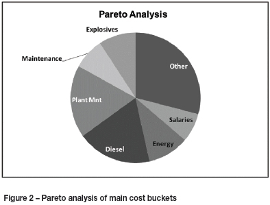
The following analysis demonstrates the complexity of the problem. For example, the cost of diesel is influenced through price fluctuations, over which the mine has no control. However, if it is influenced by production, i.e. higher production will require more diesel, but if there are better standards (fewer litres per ton produced), the mine will require less diesel than budgeted. It is therefore clear that a different approach is required to find the real drivers that will meet the requirements of a distribution that can be manipulated.

In re-examining the approach, the following alternative view of the process is proposed. The process (in a mining environment) can now be summarized as follows:

➤ The budget utilizes assets (production units) to mine and to supply ROM to the plant

➤ The plant beneficiates and delivers product to be sold.

To use any asset for continuous production, three thingsare required, namely capital, utilization, and maintenance. In using the assets, the main drivers that will influence the budget can now be stated as:

➤ Capital. Only three things can happen to capital expenditure - it may be replaced, sustained, or increased

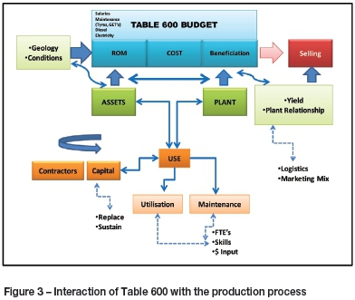
➤ Use of assets. Assets are either being used or maintained. If they are in use, they can be used productively. The level of utilization will depend on the skills level of the people and the number of full-time employees (FTEs). Both may be changed by applying more money i.e. more people can be employed, or they can be trained better. The same basic argument can be applied to maintenance. More money can be spent on better maintenance (replace before failure etc.), employing more FTEs, and/or training them better. Figure 3 shows the detail.

 

 

Plant yield (which provides the link between the budget and the geology) is one of the most important drivers in a budget, as the quantity and quality of the product drives the total income stream of a mine. In the geological environment, boreholes are drilled to set spatial parameters. As an example, for a coal mine, coal from the boreholes is analysed in a laboratory to determine a washability curve that gives the various qualities at specific densities. The information is then spatially configured through a database coupled to a geological model. The model uses different types of growth algorithms, statistical methods etc. to predict the information in-between the boreholes - normally given in a grid (or block) format. Since the predictions are not absolute but rather an approximation of the truth, this imparts a 'probability' flavour to the process. It should be noted that the interpretation of washability gives a singular deterministic value for a specific block of coal. However, as the analysis is done in a laboratory, there will be a difference in the results, as the operational procedure (i.e. production) occurs under dynamic conditions. It is sufficient to note that the yields will rarely be better than expected. The next problem is caused by the operational procedure followed in product bed-building. Production beds are normally required to conform to very strict quality specifications. It is standard practice, to build a product bed with a slightly higher than required quality, as it is easier to add low-grade material rather than above-grade in the beneficiation environment. When the bed is of too high a grade, nobody worries, and there may even be some bonuses. However, if the bed is out of specification on the 'poor' side, the company may incur large penalties or even rejection of the product by the customer. Because of this principle, and coupled to the fact that the beneficiation curve is not linear, it is common knowledge that one never gains on the upswing what is lost on the downswing. The schedule determines the time when a specific mining block will be beneficiated.

The methodology proposed here, is to take cognisance of the 'stochasticity' and to introduce variability with a triangular stochastic distribution as suggested by Clark, Reed, and Stephan (2010). With this triangular distribution, the Arena^® model will simulate operator error and variability, which will represent reality much closer than utilizing a single deterministic value. As expected, the yield will form a distribution around the budget figure.

Although the uncertainty assumed for the evaluation of the Dereköy copper deposit (Erdem et al., 2012) demonstrates a probability curve of NPV, it ignores the time component in relation to the actual mining of the deposit. This is a serious shortcoming, as a financial budget is by default a forecast of monetary flow over time. The mining operator can influence this to a large extent - for example, high-grading early on will increase the NPV, etc.

The geology and other mining conditions are given inputs to the budget. These are accessed through the mining schedule, which links time-based production outcomes to the budget. This is done with scheduling software (XPAC^®), where the yield and plant relationships that will exist sometime in the future are derived through a time-based production schedule. The resultant product mix will impact on logistics and marketing constraints if more than one product is sold. This solution may then be used to calculate the revenue or income, culminating in the final budget figure, expressed as a net profit.

The above description is a somewhat simplified version of the actual process, but based on logic and demonstrably accurate enough to deal with the myriad of confusing interrelationships that exist in such a complex environment.

Rigidity of the mine plan

The development or mining of an open pit follows very strict rules, i.e. the pit may be described in terms of a series of consecutive pit shells, governed by the need to keep the slopes at stable angles and have roads and ramps in place for access to specific mining blocks. Although some deviations are possible, for a given budget period the interrelationship between the different material types will have a fixed correlation, for example the pit slope has to be maintained, so the percentage distribution between benches will stay the same, but with increased production the slope will move faster, and with decreased production, it will move slower.

The haul truck - defining the heartbeat

A truck carries a payload that is not a fixed tonnage but may vary considerably. There are specific factors that cause this, e.g. the load-tray design, loader operator expertise, loose bulk density of the material (i.e. after blasting) and the type of material, which all vary considerably for any given pit. Overloading will lead to spillage, and exceeding the maximum carrying capability will cause damage to the truck.

A truck moves material from a given point to a fixed destination - normally from a series of mining benches to a plant or crushing facility, or in the case of overburden to a waste dump. A truck haul cycle consists of the following components: full hauling, queue at bin, tip, empty hauling, queue at loader, spot, load, and the cycle starts again.

It is clear that there is a rigidly defined or fixed number of production hours per year, day, or month during which the truck may be utilized. During this time the truck must operate not only productively, but also be maintained. Waiting times (times not spent hauling) should be as short as possible.

Probabilistic methodology

The logic component is clearly defined in the budget process. Combining this with a probabilistic approach aims to determine:

➤ What do the confidence levels look like for a given budget?

➤ Could the application of probabilistic logic influence the inherent risk of non-compliance with the budget?

➤ Will a stochastic approach allow the budget owner to establish a target probability with a higher confidence level?

To answer these questions, the impact on the budget or the achievement thereof must be simulated in a stochastic environment. The problem with this statement is that setting up the model and running it takes up to 40 minutes per run. A true stochastic simulation would therefore take approximately 2 years to complete.

Probabilistic cash flow model

From the literature it is clear that stochastic simulation is not applied to the prime financial budget, but is used to assess either the risk or the cost associated with large projects.

A systematic approach to modelling of the budget is needed that will allow simulation of results under a variety of possible scenarios. In other words, simulated net cash flow with extreme movements within the controllable budget inputs, such as fluctuations in the norms and standards that underpin the budget, is required. In summary, the model predicts the potential loss or profit in relation to the budget over a defined period, reflecting a probability distribution for which a given confidence interval can be assumed for the achievement (or non-achievement) of the budget. (Budget risks such as higher inflation, higher diesel prices, underper-forming assets, and declining revenues cannot be ignored, since for a large mine the influence of these risks may be significant enough to threaten the company's ability to fund new projects, pay dividends, and impair cash flow).

Model interaction - probabilistic methodology (Figure 4)

 

 

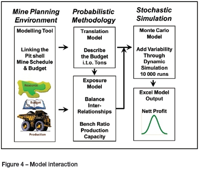
A methodology that will keep the space-time interrelationship intact, honour the integrity of the mine plan while taking cognisance of the budget complexity, and meet the simulation criteria with regard to computing time constraints is needed.

As explained, the initial phase is a modelling tool that will link the mining schedule to the budget. The Xpac^® model, which drives the tonnage schedule on which the budget is based, is used to obtain bench information for tons, hours, cycles, payload, and destination - i.e. from where (which blast block) to which plant or overburden dump.

Next, the translation model describes the budget in terms of tons. Simultaneously, the costing (ABC) model is used to give inputs to the exposure model for the different variables. The exposure model balances the bench ratios etc.

The fundamentals and statistics interact to derive a model with economic logic - in other words, a basic cash flow model underpinned by logic. The macroeconomic variables or drivers that have a significant influence on the budget performance can now be entered and distributions for the identified drivers applied. Risk is derived from random, unexpected deviations from the forecasts.

Finally, a stochastic process (an Arena^® Dynamic simulation model) is used to simulate values of the variables by randomly picking observations from their variance/covariance matrix.

Deriving the budget description in a mathematical expression

The budget / can be described from Xeras^® in terms of fixed (Fc) and variable costs (Vc). The variable costs are a function of ROM tons, which are a function of operational performance (OP).

Budget (Pareto-based) cost function f =

Fc_Other + Fc_Salaries + (Vc_Salaries x tons)

+ Fc_Energy + (Vc_Energy x tons)

+ Fc_Diesel + (Vc_Diesel x tons)

+ Fc_Plant Maintenance + (Vc_Plant Maintenance x tons)

+ Fc_Maintenance + (Vc_Maintenance x tons)

+ Fc_Explosives + (Vc_Explosives x tons)

Budget Income f = (AvePrice x tons)

ROM tons can be described by the operational performance drivers. These drivers can be described by probability distributions which can be measured and managed and influenced. The relationship between the operational performance drivers and tons can be determined with a function. The main operational performance drivers are:

➤ Maintenance (availability and utilization)

➤ Operators (FTEs, skills, production rate)

➤ Fleet units.

Stochastic simulation

The Arena^® Dynamic simulation model was used to simulate the cash flow model analysis. The objective of the model is to vary chosen business drivers in order to obtain a net cash flow distribution for the budget.

The model uses Excel^® driver inputs (per destination per bench) obtained from an Xpac^® life-of-mine schedule. Typical driver inputs like cycle times, bench ratios, payloads, fleet hours, and physical standards are read in by the model. The model then uses probability distributions to independently vary the drivers like cycle times, payloads, and fleet hours, also making provision for force majeure events and operator absence.

The model adjusts the driver values and then ensures that the fleet size and bench ratio are kept constant in order to simulate new bench tons and product tons. The model has product prices per bench, per destination, and per product, and also has the variable and fixed costs as derived from the Table 600 Budget, in order to calculate a net cost and net income.

Ten thousand variable runs of each independent driver are simulated and the values are recorded in order to apply a statistical analysis of the net profit spread using an Excel^® input sheet with built-in formulae for evaluation. Because Arena^® does not use 'time' in the sense that the scheduling model does, an extra iteration to limit the total production hours available had to be implemented. This increased the complexity of the model without influencing the stability.

The final Monte Carlo model was also expanded to be able to 'randomize' more than one parameter simultaneously so that influence on the budget of any combination of parameters can be tested . The interaction between the different environments and accompanying models is depicted in Figure 4.

Data used

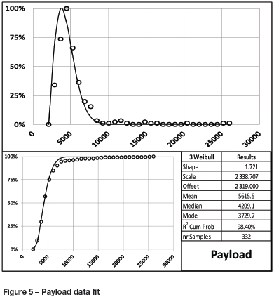
The data for the probability distributions is obtained from the mine's history through a sequel server database. Values are generated fitting Weibull distributions with an Excel^®-linked spreadsheet.

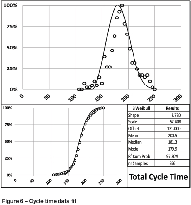
The curves fitted are three-parameter Weibull curves. The maximum likelihood estimation (MLE) method is generally considered to be the best method for estimating the curve parameters for a two-parameter Weibull curve (balancing resources and accuracy), but poor with three-parameter methods (Cousineau, 2009). Therefore the method for estimating the shape of the distribution is a modified MLE, which intelligently identifies the offset parameter before applying the MLE. The accuracy of the resulting curve has proven to be consistently adequate during testing on real data. Some results are shown below in graphical format as probability distribution and cumulative probability distribution curves.

The following are examples of curve-fitting to real data as obtained from the dispatch sequel server database: The payload distribution (depended on the material density) and total cycle times are shown. Not shown, but fitted, were: empty hauling time, spot time, queuing, loading, full haul, dump, and reassign time. From a visual inspection it is clear that the methodology applied, i.e. using a three-parameter Weibull curve-fitting technique, yields the desired results. Typical results obtained are shown in Figures 5 and 6.

 

 

 

 

Results

The following results are based on a real case study. The budget has been normalized so as not to release sensitive information. The answers are given in profit units, called net profit, and expressed as millions of rands.

In the analysis that follows, it must be borne in mind that the budget was completed at least 3 months prior to the start of the budget year. The cycle time and payload information that were used were the actual for 3 months into the budget, as well as the preceding 3 months, i.e. 6 months of real-time data. All examples refer to a large open pit mine.

Cycle and payload

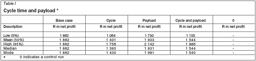
In this particular example, the mine had a problem, prior to budgeting, with the standards used cycle times. They either were under pressure not to drop the physical standards too much, or did not fully understand the implication of the trend that they were seeing, or a combination of both. It would appear that they thought that the longer cycle times could be countered by increasing the payloads that the trucks were carrying. In other words, they 'under-budgeted' on payloads.

Figures 7 and 8 show the situation. The budget was set at 1862 units (Table I). The effect of the poor cycle times at 50% results in a target of 1401 - below the budget. It is clear that the effect of the cycle time deterioration was not apparent when the budget was compiled. The strategy of countering the poor cycle time performance with loading (1933 units at 50%) is obviously not working as the increase in payload moves the target to only 1554 units compared with a budget of 1862, clearly indicating that the budget will be at risk.

 

 

 

 

Production hours (FMs)

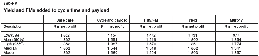
In the following example, the influence of lost production hours is examined (see Table II). A triangular distribution is deemed to be the best fit to describe this problem, as depicted in Figure 10. The mine has on average two trucks down, either through an accident or an unforeseen rebuild. Section 54 (Mine Health and Safety Act) stoppages cause a loss of on average four production days. The rest of the loss is made up of 'truck standing no operator' (dispatch code). The fit for the data is a triangular distribution with a mean of 21 340 production hours, less 10% plus 5% (these events are seen as a force majeure, hence the terminology FM.) The mean drops to 1519 against the budget of 1862, with a very narrow distribution as indicated (Figure 10).

Yield (influence)

Because yield causes a distribution around the budget line (Figures 9 and 10) it gives a target of only 1802 against the budget of 1862, as expected.

 

 

 

 

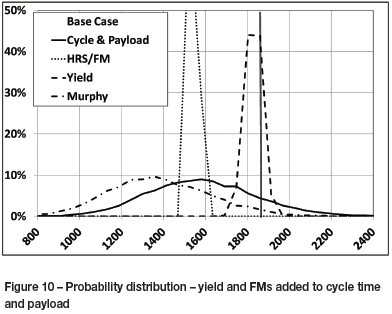
Murphy (if everything that can go wrong, goes wrong)

It is clear that if all of the above events occur, then the results (called 'Murphy') are catastrophic, with a mean of only 1345 units.

Example of capex optimization

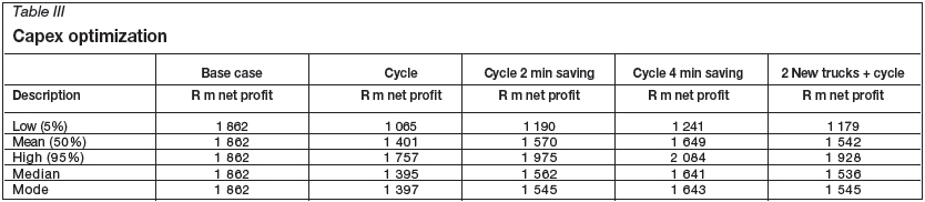
The following example demonstrates the power of the model to determine where money should be spent. In striving to achieve the budget, the mine now has the option of:

➤ Spending R10 million on upgrading the roads and improving the rolling resistance. This gives a minimum advantage of 2 minutes per cycle and a maximum of 4 minutes per cycle

➤ Alternatively, buy two additional trucks for R75 million, which will add 2 x 5500 hours = 11 000 hours for the year.

The results are compared in Table III and Figures 11 and 12.

 

 

 

 

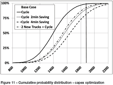
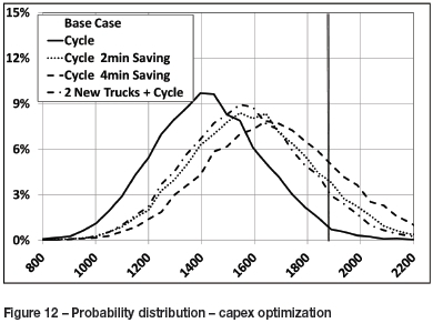
The mean moves from 1401 to 1542 with two extra trucks, or 142 units. If the cycle is adjusted by 2 minutes, (through better roads) it moves to 1570, generating 159 units. A saving of 4 minutes will give 248 units. It is clear that the better option will be to spend money on the roads instead of buying more trucks.

 

Conclusion

Monte Carlo simulation is not widely used in the industry as a budgeting tool, although there are a few examples of it being used mainly for capital budgeting and the prediction of the variations within the budget. The main reason for it not being used in the normal budget process is that the multiplication effect of the distributions of the key budget drivers leads to a spread in the budget distribution that gives an unreliable conclusion, or no conclusion at all.

The strength of the probabilistic logic model lies in the determination of the main drivers (first-order) that are independent of each other and can be influenced through the application of money. Probability logic offers a highly expressive account of deduction of where funds should be applied to optimally influence the achievement of the budget.

The probabilistic logic model circumvents the original problem of expressing the budget as a single deterministic value by using the related activity-based costing, so that when standards change the influence is clearly reflected in the new probability distribution of the budget.

The robustness of the model is guaranteed through the exploitation part of the model that directly links the deviation in standards to production. Correcting standards through the application of men, materials, or money is something that management has been trained to do and is good at. The impact and value of changing the standards are directly reflected in the probability of achieving the budget.

The stochastic model uses real data wherever possible. Hubbard (2010) makes the point that the model should only be accurate enough, and states that uncertainty can be overcome by adding more complexity to the model. This is precisely wrong in the stochastic modelling environment. The robustness of the model proposed lies in the fact that it differentiates between the primary drivers and secondary drivers which, while appearing to be important, generate so much noise that the answers become invaluable or worthless.

Testing of a real budget proved the ability of the model and the value that may be unlocked through this novel approach.

 

Acknowledgements

The authors wish to thank Professor Kris Adendorff for his valuable comments.

 

Acronyms

➤ Arena^® - Simulation software

➤ force majeure - Act of God, i.e. unforeseen and uncontrollable

➤ Murphy - Refers to Murphy's Law, an adage typically stated as 'Anything that can go wrong will go wrong'

➤ SAP^® - Enterprise software used in the industry

➤ Table 600 - A generic budget summary used in SAP^®

➤ Xeras^® - Software from the Rung suite for costing schedules

➤ XPAC^® - Scheduling software from the Runge suite, widely used in mine planning

 

References

Clark, V., Reed, M., and Stephan, J. 2010. Using Monte Carlo Simulation for a Capital Budgeting Project. Management Accounting Quarterly, vol. 12, no. 1. pp. 20-31.         [ Links ]

Cousineau, D. 2009. Nearly unbiased estimators for the three-parameter Weibull distribution with greater efficiency than the iterative likelihood method. British Journal of Mathematical and Statistical Psychology, vol. 62, part 1. pp.167-91. http://www.ncbi.nlm.nih.gov/pubmed/18177546 [Accessed 18 September 2013].         [ Links ]

Elkjaer, M. 2000. Stochastic budget simulation. International Journal of Project Management, vol. 18, no. 2. pp.139-147. http://linkinghub.elsevier.com/retrieve/pii/S0263786398000787.         [ Links ]

Erdem, Ö., Guyaguler, T., and Demirel, N. 2012. Uncertainty assessment for the evaluation of net present value : a mining industry perspective. Journal of the Southern African Institute of Mining and Metallurgy, vol. 112, no. 5. pp.405-412.         [ Links ]

Hubbard, D.W. 2010. How to Measure Anything: Finding the Value of "Intangibles" in Business. 2nd edn. Wiley.         [ Links ]

JØsang, A. 2009. Subjective Logic. Representations, vol. 171 (January). pp. 1-8. http://persons.unik.no/josang/papers/subjective_logic.pdf.         [ Links ]

US Air Force. 2007. Cost Risk and Uncertainty Analysis Handbook. Tecolote Research Inc., Golera, CA. pp. 153-178.         [ Links ]

Schragenheim, E. and Dettmer, H.W. 2000. . Simplified drum-buffer-rope. A whole system approad to high velocity manufacturing. Goal Systems International, Port Angeles, WA, USA.         [ Links ]