GENERAL PAPERS

 

Integration of imprecise and biased data into mineral resource estimates

 

 

A. Cornah^I; E Machaka^II

^IAnglo American, formerly of QG Consulting
^IIKumba Iron Ore

 

 

---

SYNOPSIS

Mineral resources are typically informed by multiple data sources of varying reliability throughout a mining project life cycle. Abundant data which are imprecise or biased or both ('secondary data') are often excluded from mineral resource estimations (the 'base case') under an intuitive, but usually untested, assumption that this data may reduce the estimation precision, bias the estimate, or both.
This paper demonstrates that the assumption is often wasteful and realized only if the secondary data are naïvely integrated into the estimation. A number of specialized geostatistical tools are available to extract maximum value from secondary information which are imprecise or biased or both; this paper evaluates cokriging (CK), multicollocated cokriging (MCCK), and ordinary kriging with variance of measurement error (OKVME).
Where abundant imprecise but unbiased secondary data are available, integration using OKVME is recommended. This re-appropriates kriging weights from less precise to more precise data locations, improving the estimation precision compared to the base case and to Ordinary Kriging (OK) of a pooled data-set. If abundant secondary data are biased and imprecise, integration through CK is recommended as the biased data are zero-sum weighted. CK consequently provides an unbiased estimate with some improvement in estimation precision compared to the base case.

Keywords: Mineral resource estimation, data integration, cokriging, ordinary kriging with variance of measurement error

---

 

 

Introduction

In mining projects it is common that the resource estimate is informed by multiple overlapping sources of 'hard' data. Sample information for the attribute(s) of interest may have been acquired from various generations and types of drilling campaigns (such as diamond, sonic, reverse circulation, or percussion). In addition, for brownfield sites, production data such as channel samples or blast-hole samples may also be available. Each data source is likely to be associated with a different level of precision and accuracy, as demonstrated by quality control metadata or twinned drill-holes. In addition, the various data sources often feature differences in sample support.

At the outset of the resource estimation process, various key decisions are required; one of these is whether all of the available hard data should be incorporated into the estimation, or whether some data should be excluded on the basis of imprecision or bias or both. Inclusion of additional data reduces the information effect (Journel and Huijbregts, 1978), but by excluding one or more data sources the practitioner judges that the benefit of that data (in terms of minimizing estimation error) is outweighed by its imprecision or bias or both. However, in practice this judgement is rarely quantified and fails to consider the various geostatistical techniques available to account for imprecision and bias during estimation.

 

Integration of imprecise or biased data

Numerous case studies concerning resource estimation based upon multiple generations of drill-hole data are documented in the literature (for recent examples see Collier et al., 2011 and Smith et al., 2011). Other authors have previously compared techniques for integrating data of different types and reliability. For example, Emery et al. (2005) compared five geostatistical techniques for integrating two subsets of error-free (assumed) and imprecise data into a resource estimate, including ordinary kriging (OK) of the pooled data-set; separate OK of each data-set and subsequent combination of the estimates by weighted average; cokriging (CK) of the two data sources; lognormal kriging with a filtering procedure; and indicator kriging to determine e-type estimates of grade. Emery et al. (2005) contend that the kriging techniques tested are not very sensitive to the level of sampling error and that the quantity of data prevails over the quality; they conclude that imprecise and unbiased measurements should never be discarded in the estimation paradigm despite their poor quality. However, Abzalov and

Pickers (2005) compared kriging with external drift (KED) and collocated cokriging (CCK) against OK for the integration of two different generations of sample assays, finding that KED and CCK significantly improved the accuracy of grade estimation when compared with conventional OK.

This paper firstly re-examines the case where imprecise but unbiased secondary data are available for incorporation into the resource estimate; the imprecise and biased case is then considered. Various techniques are trialled, including integration through CK, multicollocated cokriging (MCCK), and OK with variance of measurement error (OKVME).

CK is classically the estimation of one variable based upon the measured values of that variable and secondary variable(s). Estimation uses not only the spatial correlation of the primary variable (modelled by the primary variogram) but also the inter-variable spatial correlations (modelled by cross-variograms). By making use of data from a secondary variable(s) as well as the primary variable, CK aims to reduce estimation variance associated with the primary variable (Myers, 1982; Olea, 1999); it also seeks to enforce relationships between variables as measured within the data.

CK coincides with independent OK if all variables are sampled at all locations (isotopic sampling) and the variables of interest are also intrinsically correlated (see Wackernagel, 2003); this is a condition known as autokrigeability (Journel and Huijbregts, 1978; Matheron, 1979; Wackernagel, 2003). However, in the isotopic sampling but non-intrinsic case, real and perceived difficulties are usually deemed to outweigh the benefit of CK over OK (see Myers, 1991; Kunsch et al., 1997; Goovaerts, 1997). Various authors including Journel and Huijbregts (1978) and Goovaerts (1997) suggest that CK is worthwhile only where correlations between attributes are strong and the variable of interest is under-sampled with respect to secondary variables (heterotopic sampling) (see Wackernagel, 2003).

Even in the heterotopic sampling case, secondary data that are co-located or located near unknown primary data tend to screen the influence of distant secondary data; the high degree of data redundancy can produce large negative weights and instability within CK systems (Xu et al., 1992). In addition, fitting a positive definite linear model of coregionalization (LMC) to multiple attributes is often considered problematic (Journel, 1999), although significant improvements have been made in automated fitting routines (for example see Goulard and Voltz, 1992; Kunsch et al., 1997; Pelletier et al., 2004; Oman and Vakulenko-Lagun., 2009; Emery, 2010). Furthermore, the inference of cross-variograms is problematic in the displaced heterotopic sampling case where the sample locations of the secondary variable do not coincide with the primary variable.

In this paper CK is used to integrate dislocated heterotopic primary and secondary sample data representing the same attribute in cases where the latter is imprecise or biased or both, but spatially correlated to the former.

CCK was proposed by Xu et al. (1992) to avoid the matrix instability associated with CK discussed above. It is usually applied in cases where primary data is sparsely distributed but secondary data is quasi-exhaustively measured (for example seismic attributes in petroleum applications). Under a Markov-type screening hypothesis (Xu et al., 1992), the primary data point screens the influence of any other data point on the secondary collocated variable. This assumption allows CK to be simplified to CCK in that only the secondary data located at the estimation target is retained within the CK system; the neighbourhood of the auxiliary variable is reduced to only one point: the estimation location (Xu et al., 1992; Goovaerts, 1997). Under the Markov model the cross-covariance is available as a rescaled version of the primary covariance (Xu et al., 1992).

MCCK makes use of the auxiliary variable at the estimation location and also at sample locations where the target variable is available, but not at other locations where only the auxiliary variable is available (Rivoirard, 2001). This study investigates the possibility of integrating the secondary sample data, which represents the same attribute by MCCK.

Another alternative is to integrate data sources of varying precision using OKVME (Delhomme, 1976). The method requires that the precision of each sample incorporated into the estimation is known. The approach also requires the assumption that measurement errors represent pure nugget effect; that is, the measurement errors are non-spatial noise which is independent of the data values (see Wackernagel, 2003). The specific measurement error variance of each data point is added to the diagonal terms of the left-hand kriging matrix. The response is re-appropriation of the kriging weights in favour of sample locations with low measurement error variance and against samples with high measurement error variance. In practice it is unlikely that the precision of every measurement is known: sampling errors may be broadly assessed for each campaign based upon quality control metadata, allowing progressive penalization of progressively imprecise data. Details of procedures for measuring and monitoring precision and accuracy in geochemical data are given by Abzalov (2008, 2009).

 

Modelling

Experimentation was carried out using a two-dimensional iron ore data-set that comprises a set of exploration samples from a single geological unit configured at approximately 75 m x 75 m spacing. These samples were derived from diamond drill core and for the purpose of this experiment are assumed to be error-free; herein they are referred to as the 'primary data', Z₁.

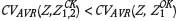
An exhaustive 'punctual ground truth' model of Fe grades within the data-set area was generated at 1 m x 1 m spaced nodes by conditional simulation (CS) of the primary data (Journel, 1974; Chilès and Delfiner, 1999). CS allows multiple images of the deposit to be generated which are realistically variable but are 'conditional' in the sense that they honour the known but limited drill-hole sampling data from the deposit. In this case, a single realization of Fe grade (which adequately represented the statistical moments of the input data) was selected from a set of 25 that were generated using the turning bands algorithm (Journel, 1974). This 'punctual ground truth' realization was averaged into 50 m x 50 m mining blocks as shown in Figure 1 to provide a 'block ground truth' (Z) against which estimations based upon the primary and secondary data could be compared.

The top left-hand plot in Figure 1 portrays the primary data locations (shown as solid black discs) and the CS realization built from this data, the histogram of Fe grades pertaining to this is shown below; the re-blocked realization is shown in the top right graphic and the histogram pertaining to this below. The figure demonstrates the key features of up-scaling from punctual to block support under the multigaussian model assumptions that underpin the CS realization (see Journel and Alabert, 1989): the range and skewness of the distribution is reduced, but the mean is preserved.

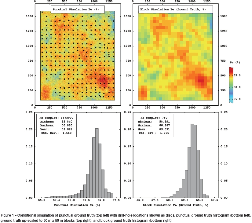
In order to provide a series of abundant secondary sample data-sets (Z₂), 'virtual' samples were extracted from the punctual ground truth. Multi-generational data sources often overlap, but are rarely exactly coincident unless they represent re-assay of older pulps or rejects. The Z₂data locations were therefore made irregular and dislocated from Z₁in order to provide a realistic representation of a multi-generational drilling campaign (the displaced heterotopic sample arrangement; see Wackernagel, 2003). Regular 25 m x 25 m locations were adjusted by easting and northing values drawn from a uniform distribution over [-3,3] to provide the Z2 extraction locations. This geometry results in Z₂ to Z₁ frequency of approximately 10:1.

Six unbiased normal error distributions were applied to the extracted Z2 samples with absolute error standard deviation ranging between 0.25 and 3 (see Figure 2), termed unbiased cases hereafter. Because the error distributions are symmetric and unbounded, imprecision has no implication with respect to bias. In addition, six positively biased error distributions centred upon absolute +1% were applied, and six negatively biased distributions centred upon absolute -1% were applied, each with the same range in (termed biased cases hereafter).

An OK block estimate incorporating the primary data only represents the base case and is compared against the block ground truth in the scatter plot shown in Figure 3.

 

 

In bedded iron ore data-sets, the Fe distribution is typically negatively skewed (see Figure 1), the data is characteristically heteroscedastic (i.e. subsets of the data show differences in variability), and the proportional effect usually exists (local variability is related to the local mean; see Journel and Huijbregts, 1978). Figure 3 indicates that the variance of estimation error is least where the local mean is greatest but increases as the local mean declines. This implies that the proportional effect exists in this data-set with local variability, and consequently estimation error, greatest in lower grade areas and least in high-grade areas. This is common in iron ore data-sets where the low-grade areas may pertain to deformed shale bands, discrete clay pods, diabase sills, or unaltered banded iron formation.

The Pearson correlation coefficient (shown as rho in Figure 3) measures the linear dependency between Zand and thus quantifies the precision of the estimate. However, following a review of the various precision metrics used in geochemical data-sets, Stanley and Lawie (2007) and Abzalov (2008) both recommend using the average coefficient of variation (CV_avr(%)) as the universal measure of relative precision error in mining geology applications:

Errors in geochemical determinations can be considered analogous to estimation errors in this case, and the CV_avr(%) metric is thus used as the basis for comparison between estimation precision in this paper. In the base case estimate shown in Figure 3, CV_AVR(Z, )0.88.

 

Analysis of imprecise but unbiased cases

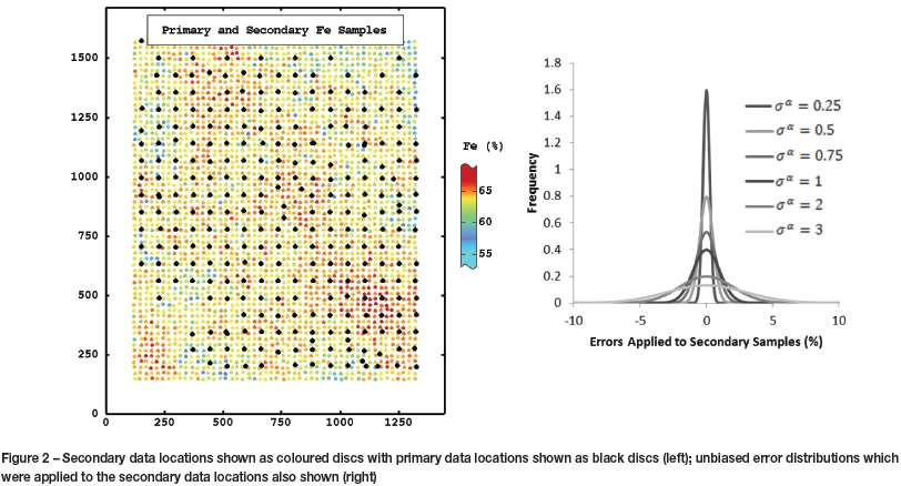
The Z₁ and unbiased but increasingly imprecise Z₂ data-sets were integrated into estimation through OK , CK , MCCK , and OKVME . Given the displaced heterotopic geometry of the data-sets, the Z₂ locations adjacent to Z₁ were migrated into collocation to allow cross-variography in CK cases, and to allow implementation of MCCK. The resulting loss of accuracy represents a compromise of these methods in the common displaced heterotopic sample geometry case and is discussed further below. The resulting estimates are quantitatively compared against the base case CV_avr(Z, ) and against each other in Figure 4.

The figure firstly shows that CV_AVR(Z,) is independent of secondly, that pooling the primary and secondary data and estimating using OK results in CV_avr (Z,)=0.56 where . Incorporating secondary samples with zero measurement error through OK clearly improves estimation precision and is therefore preferable to excluding them. However, as increases, so CVavr(Z,) also increases rapidly (indicating that estimation precision declines). Figure 4 shows that, in this particular case, where there is no benefit to including Z₂ samples in the OK estimate:

Where measurement errors are large, the OK estimate using the pooled data-set is less precise than the base case, which excludes the secondary data. In the discussed case study:

Figure 4 shows that where some improvement in estimation precision is achieved by incorporating secondary samples through CK compared to . However, in this circumstance the improvement in accuracy is not as great as that gained through

This is due to the vagaries of CK compared to OK, which were discussed above. However, as increases, the benefit of declines relative to . In this case, where CV_AVR, both of which are more precise than the base case. Where the precision of the secondary data is poorer than this, integrating it through CK is preferable to integrating it through OK. In this case:

Unlike OK, integrating the secondary data using CK provides an improvement in estimation compared to the base case in all of the cases tested:

As discussed above, MCCK is an approximation of full CK and some loss of estimation precision is to be expected in this case by the migration of data locations required by non-colocation of primary and secondary data-sets. This is evident within the results shown in Figure 4: MCCK mirrors fully the CK result, with some loss of estimation precision where However where the difference between the two approaches is negligible, suggesting that at higher levels the simplifications associated with MCCK represent a worthwhile trade-off compared to CK. In addition, integration of secondary data through MCCK is preferable to the base case in all cases that were tested:

Finally, Figure 4 shows the results of integrating secondary data through OKVME estimation . In all cases that were tested, this approach outperformed the base case:

The figure confirms that the result converges on where zero error is associated with the secondary variable:

However, as the precision of the secondary data declines, outperforms by an increasing margin; it also out-performs both and Therefore in all of the cases that were tested the following relationship holds:

To further elucidate the OKVME technique, the cumulative kriging weights allocated to each sample during the OK and OKVME estimations were recorded. The mean values for each that was tested are shown in Figure 5.

The figure firstly shows that in the case the mean cumulative OK weight that is applied to the secondary samples exceeds that applied to the primary samples; this is because the secondary samples are typically in closer proximity to block centroids than the primary samples. As the secondary samples are also more numerous than the primary samples, they are clearly more influential in the OK estimation.

The figure confirms that the OK weight is independent of this results in the rapidly increasing CV_AVR(Z, ) with increasing , as shown in Figure 4. Figure 5 also shows that where no measurement error is associated with the secondary samples, the OKVME weights converge on the OK weights. As increases the OKVME weights are rebalanced in favour of the Z₁samples. In this case, where is 0.5 or greater the mean cumulative OKVME weight assigned to Z1 samples exceeds that assigned to the Z₂ samples.

Given that in the case study Z₂ samples are significantly more numerous than Z₁, a small decrease in the mean cumulative weight applied to the former must be balanced by a larger increase in the mean cumulative weight applied to the latter, due to the requirement that the weights sum to unity.

 

Analysis of imprecise and biased cases

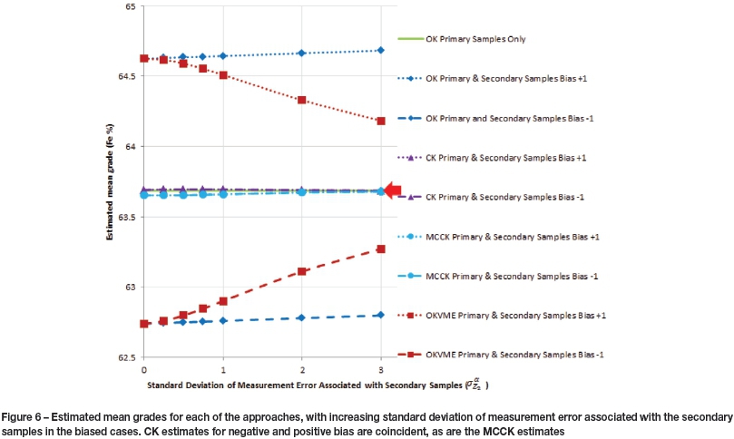
The imprecise and biased Z₂ data-sets were also integrated into estimation through OK, CK, MCCK, and OKVME. Mean estimated grades are compared against each other and the ground truth mean in Figure 6.

The figure firstly shows that the base case is unbiased with respect to the ground truth. In the , estimate weights associated with the pooled Z₁ and Z₂ samples sum to unity; consequently bias associated with Z₂ samples is directly transferred into the estimate in all cases, as is shown in Figure 6. The weights associated with the pooled Z₁ and Z₂ samples also sum to unity. However, because increasing weight is re-appropriated from Z₂ to Z₁ samples as increases, less bias is retained within the estimate in the higher cases compared to ; this is also evident in Figure 6.

In the and estimations, Z₁ sample weights sum to unity and Z₂ samples are zero-sum weighted. Figure 6 confirms that as a consequence the resulting estimations are unbiased, regardless of the bias associated with Z₂, and regardless of . Consequently, CK or MCCK represent the only viable options to integrate Z₂data that are imprecise and biased. The positive and negative bias cases are coincident for and for .

 

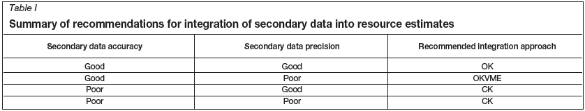
Conclusions

If precise, unbiased, and abundant secondary data are available, their basic integration through OK of a pooled data-set is pertinent (see Table I). The estimate is directly improved compared to the base case (exclusion of the secondary data) by reduction of the information effect.

However, abundant secondary data that are imprecise or biased or both are often excluded from resource estimations by practitioners, typically under an intuitive but untested assumption that inclusion will result in loss of estimation precision or that the estimation may be biased, or both. Experimentation outlined in this paper demonstrates that this may be true if the secondary data are not handled appropriately in the estimation; also that such a decision is generally wasteful.

Where imprecise but unbiased secondary data are available, it is recommended to integrate them into the estimation using OKVME (see Table I). This provides an improvement in estimation precision compared to the base case and compared to OK of a pooled data-set. CK and MCCK also provide some improvement in estimation precision compared to the base case, but do not outperform OK of a pooled data-set if abundant secondary data are relatively precise, and never out-performed OKVME in the unbiased cases that were tested.

If secondary data are associated with bias in addition to imprecision, CK is recommended as the biased data are zero-sum weighted (see Table I). CK consequently provides an unbiased estimate but with some improvement in estimation precision compared to the base case. MCCK suffers some loss of estimation precision compared to CK where the secondary data are relatively precise, but is similar to CK where the secondary data are less precise.

 

Acknowledgements

The authors would like to sincerely thank Dr Michael Harley of Anglo American, Scott Jackson of Anglo American, Dr John Forkes (independent consultant), and John Vann of Anglo American; their excellent comments and constructive criticism of earlier versions of this paper significantly improved its final content.

 

References

Abzalov M.Z. and Pickers, N. 2005. Integrating different generations of assays using multivariate geostatistics: a case study. Transactions of the Institute of Mining and Metallurgy, Section B: Applied Earth Science, vol. 114, no.1. pp. 23-32.         [ Links ]

Abzalov, M. 2008. Quality control of assay data: a review of procedures for measuring and monitoring precision and accuracy. Exploration and Mining Geology, vol. 17, no. 3-4. pp. 131-141.         [ Links ]

Abzalov, M. 2009. Use of twinned drillholes in mineral resource estimation. Exploration and Mining Geology, vol. 18, no. 1-4. pp. 13-23.         [ Links ]

Chilès, J. and Delfiner, P. 1999. Geostatistics - Modelling Spatial Uncertainty. John Wiley and Sons, Hoboken, New Jersey.         [ Links ]

Collier P., Clark G., and Smith R. 2011. Preparation of a JORC Code compliant resource statement based on an evaluation of historical data - a case study from the Panguna deposit, Bougainville, Papua New Guinea. Eighth International Mining Geology Conference, Queenstown, New zealand, 2224 August 2011. Australasian Institute of Mining and Metallurgy. pp. 409-426.         [ Links ]

Delhomme, J.P. 1976. Applications de la Theorie des variables Regionalisees Dans Les Sciences de L'Eau. Thése de Docteur - Ingénieur, Universitie Pierre et Marie Curie, Paris.         [ Links ]

Emery, X., Bertini, J.P., and Ortiz, J.M. 2005. Resource and reserve evaluation in the presence of imprecise data. CIM Bulletin, vol. 90, no. 1089. pp. 366-377.         [ Links ]

Emery, X. 2010. Iterative algorithms for fitting a linear model of coregionalization. Computers and Geosciences, vol. 36, no. 9. pp. 1150-1160.         [ Links ]

Goovaerts, P. 1997. Geostatistics for Natural Resources Evaluation. Oxford University Press.         [ Links ]

Goulard, M. and Voltz, M. 1992. Linear coregionalization model: tools for estimation and choice of cross-variogram matrix. Mathematical Geology, vol. 24, no. 3. pp. 269-286.         [ Links ]

Journel, A., 1974. Geostatistics for the conditional simulation of ore bodies, Economic Geology, vol. 69. pp. 673-688.         [ Links ]

Journel, A.G. and Huijbregts, C.J. 1978. Mining Geostatistics. Academic Press, London.         [ Links ]

Journel, A.G. and Alabert, F. 1989. Non-Gaussian data expansion in the earth sciences. Terra Nova vol. 1. pp. 123-134.         [ Links ]

Journel, A.G. 1999. Markov models for cross-covariances. Mathematical Geology, vol. 31, no. 8. pp. 955-964.         [ Links ]

Kunsch H.R., Papritz A., and Bassi F. 1997. Generalized cross-covariances and their estimation. Mathematical Geology, vol. 29, no.6. pp. 779-799.         [ Links ]

Matheron, G. 1979. Recherche de simplification dans un problem de cokrigeage. Centre de Géostatistique, Fountainebleau, France.         [ Links ]

Myers, D.E. 1982. Matrix formulation of co-kriging. Mathematical Geology, vol. 14. pp. 249-257.         [ Links ]

Myers, D.E. 1991. Pseudo-cross variograms, positive definiteness, cokriging. Mathematical Geology, vol. 23, no. 6. pp. 805-816.         [ Links ]

Olea, R. 1999. Geostatistics for Engineers and Earth Scientists. 1st edn. Oxford University Press, Oxford.         [ Links ]

Oman, S.D. and Vakulenko-Lagun, B. 2009. Estimation of sill matrices in the linear model of coregionalization. Mathematical Geosciences, vol. 41, no. 1. pp. 15-27.         [ Links ]

Pelletier, B., Dutilleul, P., Larocque, G., and Fyles, J.W. 2004. Fitting the linear model of coregionalisation by generalized least squares. Mathematical Geology, vol. 36, no. 3. pp. 323-343.         [ Links ]

Rivoirard, J. 2001. Which models for collocated cokriging? Mathematical Geology. vol. 33, no.2. pp. 117-131.         [ Links ]

Smith, D., Lutherborrow, C., Errock, C., and Pryor, T. 2011. Chasing the lead/zinc/silver lining - establishing a resource model for the historic CML7, Broken Hill, New South Wales, Australia. Eighth International Mining Geology Conference, Queenstown, New Zealand, 22-24 August 2011. Australasian Institute of Mining and Metallurgy. pp 181-189.         [ Links ]

Stanley, C.R. and Lawie, D. 2007. Average relative error in geochemical determinations: clarification, calculation, and a plea for consistency. Exploration and Mining Geology, vol. 16. pp. 265-274.         [ Links ]

Wackernagel, H. 2003. Multivariate Geostatistics. An Introduction with Applications. Springer-Verlag, Berlin.         [ Links ]

Xu, W., Tran, T.T., Srivastava, R.M., and Journel, A.G. 1992. Integrating seismic data in reservoir modeling: the collocated cokriging alternative. 67th Annual Technical Conference of the Society of Petroleum Engineers, Washington DC. Proceedings paper SPE 24742. pp. 833-842.         [ Links ]