GENERAL PAPERS

 

Technological developments for spatial prediction of soil properties, and Danie Krige's influence on it

 

 

R. Webster

Rothamsted Research, Great Britain

 

 

---

SYNOPSIS

Daniel Krige's influence on soil science, and on soil survey in particular, has been profound. From the 1920s onwards soil surveyors made their maps by classifying the soils and drawing boundaries between the classes they recognized. By the 1960s many influential pedologists were convinced that if one knew to which class of soil a site belonged then one would be able to predict the soil's properties there. At the same time, engineers began to realize that prediction from such maps was essentially a statistical matter and to apply classical sampling theory. Such methods, though sound, proved inefficient because they failed to take account of the spatial dependence within the classes.
Matters changed dramatically in the 1970s when soil scientists learned of the work of Daniel Krige and Georges Matheron's theory of regionalized variables. Statistical pedologists (pedometricians) first linked R.A. Fisher's analysis of variance to regionalized variables via spatial hierarchical designs to estimate spatial components of variance. They then applied the mainstream geostatistical methods of spatial analysis and kriging to map plant nutrients, trace elements, pollutants, salt, and agricultural pests in soil, which has led to advances in modern precision agriculture. They were among the first Earth scientists to use nonlinear statistical estimation for modelling variograms and to make the programmed algorithms publicly available. More recently, pedometricians have turned to likelihood methods, specifically residual maximum likelihood (REML), to combine fixed effects, such as trend and external variables, with spatially correlated variables in linear mixed models for spatial prediction. They have also explored nonstationary variances with wavelets and by spectral tempering, although it is not clear how the results should be used for prediction.
This paper illustrates the most significant advances, with results from research projects.

Keywords: soil, variogram, spectral analysis, gilgai, drift, mixed models, REML, non-stationary, variance.

---

 

 

Prologue

Daniel Krige's influence on soil science, and on soil survey in particular, has been profound. Yet, I suspect that Daniel did not realize it. Some 25 years ago I found myself close to his holiday home in the Cape Province and visited him there. We chatted over coffee. I told him how we were adapting and developing geostatistics for mapping soil. He was encouraging, but he was not surprised: of course the technology was applicable in our domain. What he did not know was the base from which we were starting. He could not know how Aristotelian logic, with its emphasis on classification, had constrained both soil scientists' thought and their mapping practices for more than half a century; it was not his field. So before I describe some of our achievements, I provide a little history.

I began my professional career in Africa. The year was 1957. The British Colonial Office, with the fiasco of the East African Groundnut Scheme fresh in its collective mind, recruited me to evaluate the suitability of land for agricultural development in what was then Northern Rhodesia, now Zambia. It became my job to survey and map soils for that purpose. My training in Britain, based on the identification of distinct classes of soil in a way similar to that of much geological survey at the time, ill-equipped me for what I should find. There were no obvious boundaries between one kind of soil and another on the deeply weathered rocks of the Zambian plateaux. The soil seemed to vary gradually over the landscape, though in repetitive patterns on a grand scale in sequences for which Milne (1936) had earlier coined the term 'catena'. Furthermore, the fairly dense miombo woodland in the north of country meant that one could rarely see for more than a few tens of metres, and air-photo interpretation had so far been of little help. Surveys had to be done almost entirely by sampling, and mapping by interpolation from the point observations. How was I to interpolate? There must be some method better than by hand and eye. I was no nearer to answering my question when in 1960 I was invited by Philip Beckett to pursue the matter at Oxford University alongside the Royal Engineers. The aim was to predict soil conditions at unvisited places.

Many influential pedologists at the time were convinced that if one knew to which class of soil a site belonged then one would be able to predict the soil's properties there. Beckett and I were far from convinced.

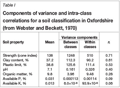
A few engineers had begun to realize that the problem was essentially statistical and were toying with a combination of classical soil maps and prediction statistics based on stratified random sampling in which the classes of the maps were the strata. Morse and Thornburn (1961) published statistics obtained by sampling agricultural soil maps in Illinois, and a year later Kantey and Williams (1962) reported results of sampling engineering soil maps in South Africa. We planned a thorough study along similar lines. We classified and mapped a large part of the Oxfordshire landscape, sampled it to a stratified random design, and measured properties of the soil. Then by analysis of variance we assessed our classification for its effectiveness in (a) diminishing the variances within the classes and (b) predicting values with acceptable precision. We also assessed maps made and sampled by several of our collaborators. We had mixed success. Our map of the Oxford region enabled us to predict the mechanical properties of the soil reasonably well. It predicted relatively poorly the soil's pH and organic matter content, and it was useless for predicting the plant nutrients in the soil. Table I from Webster and Beckett (1970) summarizes our results.

 

 

First steps

Despite our partial success, even in the most favourable situations there was substantial residual variation for which we could not account. Some we might treat as white noise, but much was evidently structural. We had not solved the problem of the catena or any other form of gradual change or trend. If we simply drew boundaries in those situations then the residuals would be spatially correlated. At about the same time, trend-surface analysis was becoming fashionable in geography and petroleum exploration, but it was unsatisfactory because (a) fluctuation in one part of a region affected the fit of the surface elsewhere and (b) the residuals were correlated so that calculated prediction variances were biased.

I was joined from Mexico by H.E. Cuanalo in 1968. He pointed out that time-series analysts have similar problems, and they treat actuality as realizations of stochastic processes to describe quantitatively fluctuations in time. Could we not do the same for soil? So we switched our thinking from the classical mode and took a leap of imagination; we should treat the soil as if it were random - against all the tenets of the day!

The Sandford transect I

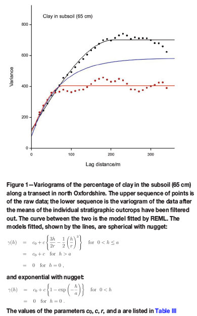
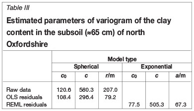
To test the feasibility of the approach we sampled the soil at 10 m intervals on a transect 3.2 km long across the Jurassic scarplands of north Oxfordshire, near Sandford St Martin, and measured several properties of the soil at each point (Webster and Cuanalo, 1975). Correlograms computed from the data showed strong spatial correlation extending to 200-250 m. This distance corresponded approximately to the average width of the outcrops and to the evident changes in soil. If we filtered out the variation due to the presence of the distinct underlying Jurassic strata we discovered that there was still spatial correlation in the residuals, though with a range of only about 80 m. Figure 1 shows an example, here with variograms rather than correlograms, for the clay content in the subsoil (±65 cm). The points on the graphs, the experimental semivariances, are computed by the usual method of moments at 10 m intervals, and the spherical functions are fitted by weighted least squares with the 'fitnonlinear' command in GenStat (Payne, 2013) with weights proportional to the numbers of paired comparisons - see also below. Table II summarizes the statistics and Table III lists the fitting parameters.

 

 

 

 

 

 

From today's viewpoint the situation seems obvious. We had two sources of variation, one from class to class, which we might treat as a fixed effect; and the other within classes, which we should treat as random. We needed a mixed model to describe it. I return to the matter below.

Nested sampling and analysis

I spent the year 1973 working with B.E. Butler, doyen of Australian pedology in the CSIRO. Our first task was to discover the spatial scale(s) on which soil properties varied on the Southern Tablelands of Australia. We sampled to a balanced spatially nested design and estimated the components of variance from a hierarchical analysis of variance (ANOVA), quite unaware that the technique had been proposed 36 years earlier by Youden and Mehlich (1937) and published in their house journal, or that it had been used by geologists Olsen and Potter (1954) and Krumbein and Slack (1956) in the intervening years, and then forgotten. We summed the components to form rough variograms and discovered that different soil properties varied on disparate scales in that complex landscape (Webster and Butler, 1976). Figure 2 shows such variograms of two of the variables. Notice that the spacings in the design increase in logarithmic progression. At about the same time Miesch (1975) had the idea of applying the same techniques for geochemistry and ore evaluation.

 

 

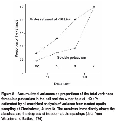
Along the bottom of the graph are the degrees of freedom with which the components are estimated. You will see that as one moves from right to left on the graph, i.e. as the scale becomes increasingly fine, the number of degrees of freedom increases twofold with each step after the first. If one wants more steps on the graph for a more refined picture, then maintaining balance by doubling the sampling soon becomes unaffordable. The increased precision at the shorter lag distances is also unnecessary. Margaret Oliver recognized the problem and sacrificed balance and analytical elegance for greater efficiency for studying the soil in the Wyre Forest of England. She and I designed a five-stage hierarchy but without doubling all branches of the hierarchy at the lowest stage, and we programmed Gower's (1962) algorithm to estimate the components of variance (Oliver and Webster, 1987). Shortly afterwards Boag and I devised an extreme form of unbalanced hierarchy with equal degrees of freedom at all stages, apart from the first, in a study of the distribution of cereal cyst nematodes in soil, and again we estimated the components of variance by Gower's method (Webster and Boag, 1992). We have since replaced Gower's method, which though unbiased is not unique, by the more efficient residual maximum likelihood method (REML) of Patterson and Thompson (1971). A full account of the procedures and guide to computer code can be found in Webster et al. (2006).

That paper, however, is not the last word; since then Lark (2011) has sought to optimize hierarchical spatial sampling. If he assumed that the variances contributed at spacings incremented in a logarithmic progression were equal, then neither the fully balanced design nor the one that distributed the degrees of freedom equally was best; the optimal design was intermediate between the two. Webster and Lark (2013) summarize the search mechanism using simulated annealing to find the optimum and the results.

The last three publications cited above should ensure that this efficient, economical way of obtaining a first rough estimate of the variogram in unknown territory will not be forgotten. It should be a part of any geostatistician's toolkit.

Gilgai and spectral analysis

A second topic in my Australian research was to investigate the repetitive spatial patterns of gilgais. Gilgais are typically shallow wet depressions a few metres across in otherwise flat plains, and their patterns seemed to be regular. The question was: is there some regularity? and if so what are its characteristics?

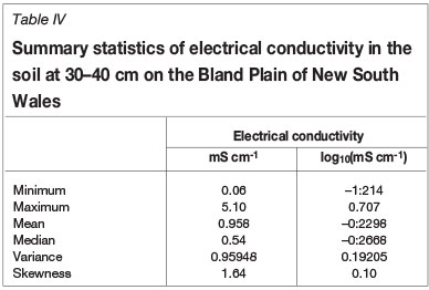
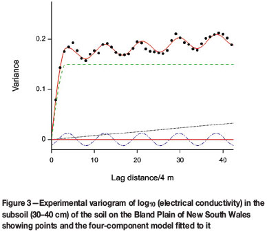
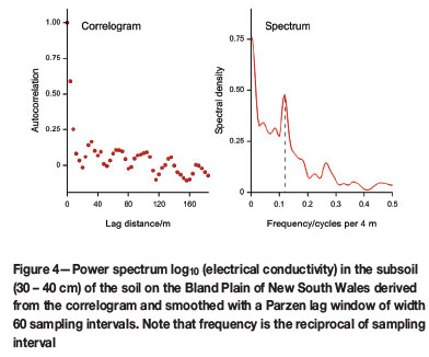
As in north Oxfordshire, I sampled the soil at regular intervals on a transect on the Bland Plain of New South Wales (Webster, 1977). The transect was almost 1.5 km long and was sampled at 4 m intervals. Table IV summarizes the statistics. The correlograms of several properties appeared wavy, and I transformed them to their corresponding power spectra. I illustrate the outcome with results for just one variable, the electrical conductivity in the subsoil (30-40 cm) converted to logarithms to stabilize the variance and with the variogram instead of the correlogram (Figure 3). The function fitted to the experimental variogram comprises four components, namely nugget, spherical, linear, and periodic. Figure 4 shows the spectrum computed with a Parzen lag window of width 60 sampling intervals. Notice the strong peak at approximately 0.12 cycles corresponding to the wavelength of 34 m in the model fitted to the variogram.

 

 

 

 

 

 

The patterns are two-dimensional, of course, and one would like to extend the above analysis in two dimensions. Despite the remark above, sampling the soil at sufficient places for such analysis was prohibitively expensive. An alternative was to analyse aerial photographic images of the Bland Plain, on which the gilgais appear typically as roughly circular dark patches on a paler background. Milne et al. (2010) took this approach.

But how could we use this intelligence to interpolate?

Perhaps the most significant event during my sojourn in Australia occurred a week or so before I was due to leave. A complete stranger breezed into my office without a by-your-leave and asked me bluntly, 'What's this kriging?'. I had never heard the term before, and rather than plead complete ignorance I played for time. Who was this intruder? and why did he ask? He was Daniel Sampey, a mining geologist. I let him talk, which he did for about 20 minutes. He told me of a certain Professor Krige and Georges Matheron, of the theory of regionalized variables and of its application in geostatistics. Then, clearly disappointed that I knew even less than he did, he left as abruptly as he had arrived. His parting shot was that as I was about to return to Britain I should visit Leeds University, where mining engineers knew a thing or two. In those 20 minutes I realized that my problem of spatial prediction of soil conditions at unvisited places had been solved, at least in principle, and in general terms I understood how. On my return to Britain I contacted Anthony Royle at Leeds. He amplified what Daniel Sampey had told me, and he generously gave me a copy of his lecture notes on the subject and some references to the literature, including Matheron's (1965) seminal thesis.

Back in Oxford I was joined by Trevor Burgess, a young mathematician. Together we turned Matheron's equations into algorithms and the algorithms into computer code. Our first scientific papers appeared in 1980 (Burgess and Webster, 1980a, 1980b; Webster and Burgess, 1980). They were the first to describe for soil scientists the variogram as we know it today and the first to display maps of soil properties made by kriging. It is from there that geostatistics in soil science burgeoned to become a branch of science with its own identity, pedometrics, and its magazine Pedometron (http://pedometrics.org/?page id=33 for the latest issue).

 

Soil: an ideal medium for geostatistics

Soil is almost the ideal medium for practical geostatistics. It forms a continuous mantle over large parts of the Earth's land surface. Access is easy over much of that, so that sampling at the working scale of the individual field, farm, or estate can be cheap. Some of soil's most important properties, such as pH, concentrations of the major plant nutrients and trace elements, salinity, and pollutant heavy metals are also cheap to measure nowadays: pedometricians need not be short of data for these variables, and from large databases they can estimate spatial covariance functions or variograms accurately. The statistical distributions of these properties are in most instances 'well-behaved' in that they are either close to normal (Gaussian) or to lognormal, so that in the latter situation a simple transformation to logarithms makes analysis straightforward and efficient. Furthermore, although the laws of physics must be obeyed as soil is formed, the numerous processes that operate and have operated in combination over many millennia to form the present-day soil have produced a complexity that is indistinguishable from random (Webster, 2000). So, we can often treat soil as the outcome of random processes without harming our professional reputations.

It is a small step from there to assume that soil variables are intrinsically stationary. In the conventional notation

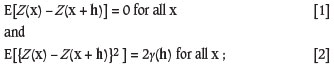
where Z(x)and Z(x + h)denote random variables at places x and x + h, and vector h is the separation, or lag, between them in the two dimensions of soil survey. Ordinary kriging follows. From the 1980s onwards it has become the workhorse of geostatistics in surveys, not only of soil itself but also in the related fields of agronomy, pest infestation, and pollution; there are hundreds of examples of its application described in the literature. It is proving to be valuable in modern precision agriculture in particular - see Oliver (2010) and the topics therein.

Disjunctive kriging required a somewhat larger advance in technique. Matheron (1976) formulated it for selection in mining. Pedologists saw in it the means of estimating and mapping the probabilities of nutrient deficiencies over land grazed by cattle and sheep (Webster and Oliver, 1989; Webster and Rivoirard, 1991) and of contamination by potentially toxic metals (von Steiger et al., 1996). In both situations thresholds are specified to trigger action. In the first, the thresholds are minimum concentrations of available trace elements such as copper and cobalt. If the soil contains less than these thresholds then stock farmers are advised to supplement their animals' feed or to add salts of the elements to their fertilizers. However, kriged estimates of concentrations are subject to error, and farmers do not want to risk deficiencies by taking those estimates at face value. They want in addition estimates of the probabilities, given the data, that patches of ground are deficient. In the second situation the thresholds are maxima, in excess of which authorities must clean up or restrict access. Again, estimated concentrations are more or less erroneous, and an authority will wish to have estimates of the probabilities of excess before spending taxpayers' money on unnecessary remediation or risking poisoning people or grazing animals by doing nothing.

Nonlinear modelling of variograms

Throughout the 1980s one of the most serious stumbling blocks in practical geostatistics was the lack of software in the public domain for fitting models to sample variograms. Many practitioners fitted models by eye, and they defended their practice with vigour. In some instances, estimated semivariances fell neatly on smooth curves that matched one or other of the standard valid variogram functions, and in those circumstances the practice was reasonable. But in many other situations, choosing and fitting functions to experimental variograms were, and remain, problematic. Some experimental variograms are erratic, usually because they are derived from rather sparse data. In some the numbers of paired comparisons vary greatly so that it is hard to know how to weight the points on graphs. The variation can be strongly anisotropic, so that again one cannot see what models might fit. And there can be combinations of these.

All of the popular functions, apart from the unbounded linear model, contain nonlinear distance parameters, and these cannot be estimated by ordinary least-squares regression. Some, such as the exponential and power functions, can be re-parameterized so that they are linear. Others, such as the spherical and related functions, cannot; they must be estimated by numerical approximation, and doing that requires expertise in numerical analysis. Rothamsted had that expertise; Ross (1987) had written his program, MLP, for nonlinear estimation, and we soil scientists used it to advantage for fitting models to experimental variograms (McBratney and Webster, 1986). The algorithms were incorporated in GenStat, Rothamsted's general statistical program, now in its 16th release (Payne, 2013), to provide the facilities for estimating and modelling spatial covariances completely under the control of the practitioner and with transparent monitoring of the processes. These facilities include the choice of steps, bins and maximum lags; the robust estimates of Cressie and Hawkins (1980), Dowd (1984), and Genton (1998) in addition to the usual method of moments; and variable weighting according to the expected values, as suggested by Cressie (1985). They include also the linear model of coregionalization for two or more random variables.

The facilities are readily called into play from menus. Alternatively they can be built into programs in the GenStat language, so that one can proceed from raw data, via their screening, distributions, and transformation, variography, kriging and cross-validation, to final output as gridded predictions, back-transformed if necessary, and their variances ready for mapping. GenStat (http://www.vsni.co.uk/software/genstat) is immensely powerful and is available in the public domain for a modest price.

Statistical modelling is no longer novel, and it has largely replaced fitting models by eye. Unfortunately, the pendulum has swung too far towards automation. Too often, modelling is now a blinkered push-button exercise in a geographic information system applied with little understanding or control and no facilities for monitoring.

 

Where are we now? Mixed models incorporating trend and other knowledge

Although the assumption of intrinsic stationarity has seemed, and continues to seem, easily satisfied there are two situations in which it is not satisfactory. The first is where there is geographic trend - 'drift' in the geostatistical jargon - and for which Matheron (1969) devised universal kriging. Universal kriging itself requires no more than an augmentation of the ordinary kriging system. Obtaining a valid estimate of the variogram of the random component of variation is more difficult, because what is required is the variogram of the residuals from the drift, and one cannot know what the residuals are until one has correctly identified the drift. Webster and Burgess (1980) recognized the situation, and to map the soil's electrical resistivity over an archaeological site that had been sampled on a dense grid they programmed the algorithms set out by Olea (1975) for the purpose.

Trend is a kind of knowledge in addition to the sample data. There are other kinds of additional knowledge about soil. The variable of interest, the target variable, might be related to one or more other variables that the pedologist knows or can measure cheaply at the prediction points. Or, as at Sandford mentioned above, there might already be a classification of the region that could partition the variance. How should one take this knowledge into account?

For some years pedologists answered with a pragmatic approach; they called it 'regression kriging'. They regressed by ordinary least squares (OLS) the target variables on the predictors, which could be the geographic coordinates for trend, the ancillary variables they measured, or the classes of the regions being mapped. They estimated variograms of the OLS residuals, kriged the residuals, and then added back the estimates from the regression equations at the prediction sites - see, for example, Odeh et al. (1995). The predictions are unbiased, but the prediction variances are underestimated, partly because the variograms are biased (Cressie, 1993) and partly because there is no valid way of combining the errors from the kriging and the OLS regressions. The problem was to estimate simultaneously the regression or deterministic component with minimum variance and the random residuals from the regression without bias, and then to sum the predictions of the deterministic and random variation at unsampled sites with known minimized variance. The solution, pointed out by Stein (1999), was to use maximum likelihood methods and to obtain what he called the empirical best linear unbiased predictor (E-BLUP). The basic maximum likelihood technique can be biased; residual maximum likelihood (REML) is not, and soil scientists, especially my colleague Murray Lark and co-workers, are now at the forefront among geostatisticians in its application.

The basic model underlying the E-BLUP is the linear mixed model:

in which the vector w,with K+1 columns, contains the K+1 elements 1; x₁; ... ; xkof the regression function and β contains the coefficients. The quantity ε(x)is the random residual from the regression. It is assumed to be second-order stationary with mean zero and covariance function C(h), which, because of that assumption, has the equivalent variogram ϒ(h)= C(0)- C(h).Its parameters are typically a nugget variance, c0, a structural variance, c, and a distance parameter, a, which we may denote in short by θ = (c₀, c, a}.

One finds values for the parameters in θ numerically by maximizing the log-likelihood of the residuals given the data: L [θ |z (X_d)]. Having found them, one then estimates the coefficients in β by generalized least squares, and with both sets of values known one can proceed to the kriging for prediction with its variances. Webster and Oliver (2007, pp. 200-202) provide the details. In 2006 Lark et al. (2006) called the technique 'state of the art', and though their solution by simulated annealing was still in the research phase, they showed the way forward. Now, with facilities in the public domain in SAS (http://support.sas.com/documen-tation), GenStat (Payne, 2013), and R (R Core Development Team, 2010; Pinheiro et al., 2013), for example, it can be applied as best practice.

Lark et al. (2006) illustrated their solution by kriging the soil's water content in a field with a strong trend. Later, Webster and Oliver (2007) incorporated both trend and an external drift variable - the apparent electrical conductivity of the soil - to predict and map the soil's sand content in another field. The comparisons they made of the variograms obtained using REML with those of the raw data and the OLS residuals are instructive, and I summarize them below.

Drift at Yattendon

Oliver and Carroll (2004) sampled a 23 ha field on the Chalk downland of southern England, and they measured, among other variables, the percentage of sand in the topsoil (0-15 cm) at 230 places. Their map in pixel form showed a strong regional trend. In addition they measured the apparent electrical conductivity, ECa, of the soil. In this field the ECa and the sand content are linearly related, and so one can treat the ECa as an external drift variable when predicting the proportion of sand. Webster and Oliver (2007) compared four treatments of the data:

(a) Analysis of the raw data

(b) Ordinary least-squares regression on the spatial coordinates

(c) REML to incorporate spatial trend

(d) REML to incorporate both spatial trend and ECa as external drift.

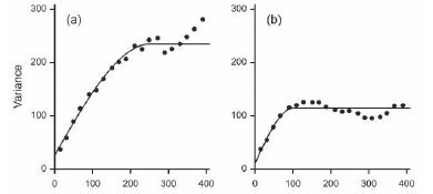
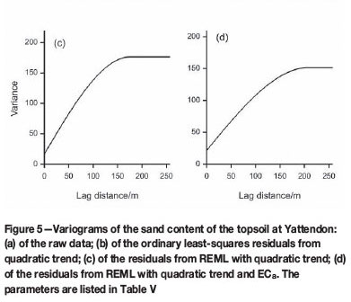
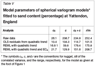
Figure 5 shows the variograms from the four treatments, and Table V lists the values of parameters of the spherical models fitted to them. The variogram of the raw data, Figure 5(a), increases to an apparent sill at a lag distance of approximately 200 m, and then increases beyond with ever-increasing gradient. The latter increase is characteristic of long-range trend. If one fits a quadratic trend surface by OLS regression and then models the variogram of the residuals one obtains Figure 5(b). Evidently the residuals are much less variable than the raw data, but they are also autocorrelated, and so the OLS regression gives a faulty representation of the truth. Figure 5(c) shows the REML variogram of the residuals with the quadratic trend fitted as a deterministic (fixed) effect. Its sill at 176.4%² is substantially larger than that of the OLS residuals in Figure 5(b). By taking into account the additional knowledge of the relation between sand content and ECa as external drift in the REML analysis one obtains the variogram shown in Figure 5(d), now with a sill of only 151.6%².

 

 

 

Webster and Oliver (2007) went on to map the sand content by punctual kriging from the data at the nodes of a fine grid of 5 m x 5 m using these variograms. The maps of the predicted values were similar, as might be expected because kriging is so robust. The kriging variances differed substantially. Those for ordinary kriging from the raw data were quite the largest; they had a mean of 63.2%². The mean variance for the OLS residuals was 52.0%², which we know to be an underestimate. That for the universal kriging, i.e. incorporating the spatial coordinates only, item (c) above, was 53.5%², and the mean for kriging with the external ECa in addition, item (d), was 48.2(%)². The example shows that the more pertinent information we have the more accurate are our predictions.

The Sandford transect II

The analysis above of the Sandford transect also used what we know about the environment, in that instance, the stratigraphy of the rocks beneath the soil as represented by the geological map. We may criticize it for the same reasons as we now criticize the early regression kriging based on the simple OLS residuals: the sampling was at regular intervals, not random, and so the within-class variances would be biased and perhaps the mean values also. Murray Lark, whom I thank, has kindly re-analysed the data based on the model of Equation [3], but now with β containing the mean value of the stratigraphic class to which position x belongs and w taking the value 1 if x belongs to that class. So again we use REML to find both the class means and the variogram of the residuals.

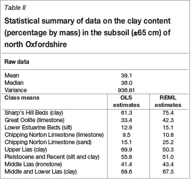
Table II lists the mean values as estimated both by ordinary least squares and by REML. The differences among the latter are highly significant statistically; the Wald statistic is 33.12, which, with 8 degrees of freedom, gives a probability of < 0:0001 for the null hypothesis. The best-fitting variogram of the residuals estimated by REML turns out to be exponential with parameter values listed in Table III. I have plotted it on the same graph as the variograms of the raw data and OLS residuals to show the comparisons in Figure 2. Its sill (c₀ + c = 582.4%²) is substantially larger than that (c₀ + c = 404:8%²) of the OLS residuals. It has a different shape from the first two, and its effective range (3 x 67.3 = 201.9 m) is comparable to the range (207.0 m) of the variogram of the raw data and much larger than that of the OLS residuals (79.2 m).

 

Nonstationary variances

A more intractable stumbling block in the spatial prediction of soil properties is that of nonstationary variances. The field pedologist knows well that some parts of a landscape are more variable than others: for example, the flood plain of a braided river does not vary in the same way or on the same spatial scale as the river's higher catchment. At Sandford the soil seemed not to vary equally on all sedimentary outcrops, and Lark and Webster (1999) introduced wavelets into soil science to investigate the matter.

A wavelet is a function that varies within a narrow window and is constant at zero outside. The window is moved step by step, i.e. translated, over the field of data, and at each position it is convolved with the data in the window to obtain its coefficient. The window can be also be dilated and again translated so that a new set of coefficients are obtained at a different scale. By plotting the results against spatial position one can see where and on what spatial scales the variance changes (e.g. Lark and Webster, 2001; Milne et al., 2011). Milne et al. (2010) also analysed aerial photographs of the gilgai patterns on the Bland Plain. Their results accorded well with, and augmented, those from the earlier spectral analysis above.

What is not yet clear is how we should take into account nonstationary variance in prediction, unless we have abundant data and can segment fields of data into zones of stationary variance. Some progress has been made by Paciorek and Schervish (2006) using a new class of nonstationary covariance functions, and by Haskard et al. (2010), who combined the linear mixed model with spectral tempering. This should be a matter of further research in the years to come.

 

Epilogue

We soil scientists are greatly indebted to Daniel Krige. Perhaps without his realizing, it was on his pioneering technology that we built and advanced in our own field; the technology and the ideas behind it released us from the constraining mind-set of earlier years and opened up a whole new field of endeavour -pedometrics. We should thank also Daniel Sampey; I shall not forget him. Who knows how much longer we should have groped at snail's pace towards the solution of our problem of spatial prediction had he not burst into my office in Australia that day 40 years ago? Finally, we should recognize the recent achievements of Murray Lark. His penetrating study of drift in its various forms, its estimation as part of the linear mixed model, and his clear and convincing writing (e.g. Lark 2012) have set soil scientists on a new and sound course in regional prediction and mapping - see, for example, the papers by Philippot et al. (2009) and Villanneau et al. (2011). Furthermore, with packages for the analysis now in the public domain we have no excuse for inferior practice.

 

References

Burgess, T.M. and Webster, R. 1980a. Optimal interpolation and isarithmic mapping of soil properties. I. The semivariogram and punctual kriging. Journal of Soil Science, vol. 31. pp. 315-331.         [ Links ]

Burgess, T.M. and Webster, R. 1980b. Optimal interpolation and isarithmic mapping of soil properties. II. Block kriging. Journal of Soil Science, vol. 31. pp. 333-341.         [ Links ]

Cressie, N. 1985. Fitting variogram models by least squares. Journal of the International Association of Mathematical Geology, vol. 17. pp. 563-575.         [ Links ]

Cressie, N.A.C. 1993. Statistics/or Spatial Data. Revised edition. John Wiley & Sons, New York.         [ Links ]

Cressie, N. and Hawkins, D.M. 1980. Robust estimation of the variogram. Journal of the International Association of Mathematical Geology, vol. 12. pp.115-125.         [ Links ]

Dowd, P.A. 1984.The variogram and kriging: robust and resistent estimators. Geostatisticsfor Natural Resources Characterization. Verly, G., David, M., Journel, A.G., and Marechal, A. (eds). D. Reidel, Dordrecht. pp. 91-106.         [ Links ]

Genton, M.G. 1998. Highly robust variogram estimation. Mathematical Geology, vol. 30. pp. 213-221.         [ Links ]

Gower, J.C. 1962. Variance component estimation for unbalanced hierarchical classification. Biometrics, vol. 18. pp. 168-182.         [ Links ]

Haskard, K.A., Welham, S.J., and Lark, R.M. 2010. A linear mixed model with spectral tempering of the variance parameters for nitrous oxide emission rates from soil across an agricultural landscape. Geoderma, vol. 159. pp. 358-370.         [ Links ]

Kantey, B.A. and Williams, A.A.B. 1962. The use of engineering soil maps for road projects. Transactions of the South African Institute of Civil Engineers, vol. 4. pp. 149-159.         [ Links ]

Krumbein, W.C. and Slack, H.A. 1956. Statistical analysis of low-level radioactivity of Pennsylvanian back fissile shale in Illinois. Bulletin of the Geological Society of America, vol. 67. pp. 739-762.         [ Links ]

Lark, R.M. 2011. Spatially nested sampling schemes for spatial variance components: scope for their optimization. Computers and Geosciences, vol. 37. pp. 1633-1641.         [ Links ]

Lark, R.M. 2012. Towards soil geostatistics. Spatial Statistics, vol. 1. pp. 92-99.         [ Links ]

Lark, R.M., Cullis, B.R., and Welham, S.J. 2006. On the prediction of soil properties in the presence of spatial trend: the empirical best linear unbiased predictor (E-BLUP) with REML. European Journal of Soil Science, vol. 57. pp. 787-799.         [ Links ]

Lark, R.M. and Webster, R. 1999. Analysis and elucidation of soil variation using wavelets. European Journal of Soil Science, vol. 50. pp. 185-206.         [ Links ]

Lark, R.M. and Webster, R. 2001. Changes in variance and correlation of soil properties with scale and location: analysis using an adapted maximal overlap discrete wavelet transform. European Journal of Soil Science, vol. 52. pp. 547-562.         [ Links ]

Matheron, G. 1965. Les variables regionalisees et leur estimation. Masson, Paris.         [ Links ]

Matheron, G. 1969. Le krigeage universel. Cahiers du Centre de Morphologie Math'ematique, No 1. Ecole des Mines de Paris, Fontainebleau.         [ Links ]

McBratney, A.B. and Webster, R. 1986. Choosing functions for semi-variograms of soil properties and fitting them to sampling estimates. Journal of Soil Science, vol. 37. pp. 617-639.         [ Links ]

Miesch, A.T. 1975. Variograms and variance components in geochemistry and ore evaluation. Geological Society of America Memoir, vol. 142. pp. 192-207.         [ Links ]

Milne, G. 1936. Normal erosion as a factor in soil profile development. Nature (London), vol. 138. pp. 548-549.         [ Links ]

Milne, A.E., Webster, R., and Lark, R.M. 2010. Spectral and wavelet analysis of gilgai patterns from air photography. Australian Journal of Soil Research, vol. 48. pp. 309-325.         [ Links ]

Milne, A.E., Haskard, K.A., Webster, C.P., Truan, I.A., Goulding, K.W.T., and Lark, R.M. 2011. Wavelet analysis of the correlations between soil properties and potential nitrous oxide emission at farm and landscape scales European Journal of Soil Science, vol. 62. pp. 467-478.         [ Links ]

Morse, R.K. and Thornburn, T.H. 1961. Reliability of soil units. Proceedings of the 5th International Conference on Soil Mechanics and Foundation Engineering, vol. 1. Dunod, Paris. pp. 259-262.         [ Links ]

Olea, R.A. 1975. Optimum Mapping Techniques using Regionalized Variable Theory. Series on Spatial Analysis, no 2. Kansas Geological Survey, Lawrence, Kansas.         [ Links ]

Oliver, M.A. (ed.) 2010. Geostatistical Applications for Precision Agriculture. Springer, Dordrecht.         [ Links ]

Oliver, M.A. and Carroll, Z.L. 2004. Description of Spatial Variation in Soil to Optimize Cereal Management. Project Report 330. Home-Grown Cereals Authority, London.         [ Links ]

Oliver, M.A. and Webster, R. 1987. The elucidation of soil pattern in the Wyre Forest of the West Midlands, England. II. Spatial distribution. Journal of Soil Science, vol. 38. pp. 293-307.         [ Links ]

Olsen, J.S. and Potter, P.E. 1954. Variance components of cross-bedding direction in some basal Pennsylvanian sandstones of the Eastern Interior Basin: statistical methods. Journal of Geology, vol. 62. pp. 26-49.         [ Links ]

Paciorek, C.J. and Schervish, M.J. 2006. Spatial modelling using a new class of nonstationary covariance functions. Environmetrics, vol. 17. pp. 483-506.         [ Links ]

Patterson, H.D. and Thompson, R. 1971. Recovery of inter-block information when block sizes are unequal. Biometrika, vol. 58. pp. 545-554.         [ Links ]

Payne, R.W. (ed.). 2013. The Guide to GenStat Release 16 - Part 2 Statistics. VSN International, Hemel Hempstead, UK.         [ Links ]

Philippot, L., Bru, D., Saby, N.P.A., Cuhel, J., Arrouays, D., Simek, M., and Hallin, S. 2009. Spatial patterns of bacterial taxa in nature reflect ecological traits of deep branches of the 16S rRNA bacterial tree. Environmental Microbiology, vol. 11. pp. 3096-3104.         [ Links ]

Pinheiro, J., Bates, D., DebRoy, S., Sarkar, D., and The R Development Core Team. 2013. nlme: Linear and Nonlinear Mixed Effects Models. R package version 3.1-110.         [ Links ]

R Development Core Team. 2010. R: A Language and Environment for Statistical Computing. R Foundation for Statistical Computing, Wien. ISBN 3-90005107-0. http://www.R-project.org/        [ Links ]

Ross, G.J.S. 1987. MLP User Manual. Numerical Algorithms Group, Oxford.         [ Links ]

Villanneau, E.J., Saby, N.P.A., Marchant, B.P., Jolivet, C.C., Boulonne. L., Caria, G., Barriuso, E., Bispo, A., Briand, O. and Arrouays, D. 2011. Which persistent organic pollutants can we map in soil using a large spacing systematic soil monitoring design? A case study in Northern France. Science of the Total Environment, vol. 409. pp. 3719-3731.         [ Links ]

Von Steiger, B., Webster, R., Schulin, R., and Lehmann, R. 1996. Mapping heavy metals in polluted soil by disjunctive kriging. Environmental Pollution, vol. 94. pp. 205-215.         [ Links ]

Webster, R. 1977. Spectral analysis of gilgai soil. Australian Journal of Soil Research, vol. 15. pp. 191-204.         [ Links ]

Webster, R. 2000. Is soil variation random? Geoderma, vol. 97. pp. 149-163.         [ Links ]

Webster, R. and Beckett, P.H.T. 1970. Terrain classification and evaluation using air photography: a review of recent work at Oxford. Photogrammetria, vol. 26. pp. 51-75.         [ Links ]

Webster, R. and Boag, B. 1992. Geostatistical analysis of cyst nematodes in soil. Journal of Soil Science, vol. 43. pp. 583-595.         [ Links ]

Webster, R. and Burgess, T.M. 1980. Optimal interpolation and isarithmic mapping of soil properties. III. Changing drift and universal kriging. Journal of Soil Science, vol. 31. pp. 505-524.         [ Links ]

Webster, R. and Butler, B.E. 1976. Soil survey and classification studies at Ginninderra. Australian Journal of Soil Research, vol. 14. pp. 1-26.         [ Links ]

Webster, R. and Cuanalo de la C., H.E. 1975. Soil transect correlograms of north Oxfordshire and their interpretation. Journal of Soil Science, vol. 26. pp. 176-194.         [ Links ]

Webster, R. and Lark, R.M. 2013. Field Sampling for Environmental Science and Management. Routledge, London.         [ Links ]

Webster, R. and Oliver, M.A. 2007. Geostatistics for Environmental Scientists. 2nd edn. John Wiley & Sons, Chichester.         [ Links ]

Webster, R. and Rivoirard, J. 1991. Copper and cobalt deficiency in soil: a study using disjunctive kriging. Cahiers de Geostatistique, Compte-rendu des Journees de Geostatistique. Volume 1. Ecole des Mines de Paris, Fontainebleau, pp. 205-223.         [ Links ]

Webster, R., Welham, S.J., Potts, J.M., and Oliver, M.A. 2006. Estimating the spatial scale of regionalized variables by nested sampling, hierarchical analysis of variance and residual maximum likelihood. Computers and Geosciences, vol. 32. pp. 1320-1333.         [ Links ]

Youden, W.J. and Mehlich, A. 1937. Selection of efficient methods for soil sampling. Contributions of the Boyce Thompson Institutefor Plant Research, vol. 9. pp. 59-70.         [ Links ]