DANIE KRIGE COMMEMORATIVE EDITION - VOLUME III

 

Application of Direct Sampling multi-point statistic and sequential gaussian simulation algorithms for modelling uncertainty in gold deposits

 

 

Y. van der Grijp^{I, II}; R.C.A. Minnitt^II

^IContinental Africa - Geology Technical Services, AngloGold Ashanti. University of the Witwatersrand
^IISchool of Mining Engineering, University of the Witwatersrand

 

 

---

SYNOPSIS

The applicability of a stochastic approach to the simulation of gold distribution to assess the uncertainty of the associated mineralization is examined. A practical workflow for similar problems is proposed. Two different techniques are explored in this research: a Direct Sampling multi-point simulation algorithm is used for generating realizations of lithologies hosting the gold mineralization, and sequential Gaussian simulation is applied to generate multiple realizations of gold distributions within the host lithologies. A range of parameters in the Direct Sampling algorithm is investigated to arrive at good reproducibility of the patterns found in the training image. These findings are aimed at assisting in the choice of appropriate parameters when undertaking the simulation step. The resulting realizations are analysed in order to assess the combined uncertainty associated with the lithology and gold mineralization.

Keywords: Direct Sampling, multi-point statistics, MPS simulation, training image, uncertainty in gold deposits.

---

 

 

Introduction

Traditionally, grade distribution in an orebody is modelled by creating a block model with a single version of geological domaining that in turn is populated with a single version of mineral grade distribution. Such a deterministic representation of reality conveys an impression that the size, geometry, and spatial position of geological units are perfectly known. If the density of the available data is such that the model can be inferred with high confidence, the approach is acceptable, but problems arise when data is widely spaced, interpretations are ambiguous, and multiple scenarios can be inferred with equal validity (Perez, 2011). Stochastic simulation, on the other hand, is used to generate multiple equiprobable realizations of a variable.

This study uses two approaches to stochastic modelling: namely, Direct Sampling (DS) for simulating lithology as geologically stationary domains, and sequential gaussian simulation (SGS) for simulating multiple realizations of grade distribution (Goovaerts, 1997) within the simulated lithologies. DS is one of many algorithms based on multiple-point statistics (MPS) and has as its basis a training image (TI). The training image is a conceptual representation of how random variables are jointly distributed in space, be they continuous or categorical variables. It portrays a model of geological heterogeneity on which further MPS simulation is based (Caers, 2011). While a two-point simulation aims at generating realizations that honour the data and the variogram model, an MPS simulation generates realizations that honour the data and the multi-point structures present in the TI (Remy, 2009).

A number of MPS algorithms have been developed in the last two decades, after the concept was first introduction by Guardiano and Srivastava in 1993 (Guardiano,1993). In 2002, Strebelle proposed the snesim algorithm for simulation of categorical variables. It utilized a 'search tree' structure to store conditional probabilities of data events which were extracted later during simulation. The snesim algorithm was computationally demanding, which made it prohibitive for simulation of large models. The Filtersim algorithm (Zhang et al., 2006; Wu et al., 2008) accommodated both continuous and categorical variables, as well as improved the computational demands by simulating batches of pixels rather than one pixel at a time. The IMPALA algorithm (Straubhaar et al., 2011) used lists instead of trees, which reduced the memory requirements by allowing parallelization; however, it was still computationally demanding. In 2007, Arpat and Caers introduced the SIMPAT algorithm, which used distance functions to calculate similarity between the TI and conditioning data events.

Multi-dimensional scaling, MDS, (Honarkhah and Caers, 2010) and the CCSIM method (Tahmasebi et al., 2012) are other examples of MPS algorithms (Rezaee, 2013).

The DS algorithm is similar to other techniques in the way it uses the principle of sequential simulation. The difference lies in the way the conditional cumulative distribution function for the local data event is computed (Mariethoz et al., 2013). Rather than storing the TI probabilities in a catalogue prior to simulation, the algorithm directly scans and samples the TI in a random fashion while conditioning to the data event d_n.It uses dissimilarity distances between the d_n and TI patterns. For each node x in the simulation grid, the TI is randomly scanned for matching patterns of nodes denoted y. A measure of satisfying the degree of 'matching' is determined by a user-defined distance threshold, which takes a range of values between 0 and 1 . As soon as a TI pattern that matches the data event d_nexactly or within the defined threshold is found, the value of the central node of such TI pattern is pasted at location x.

The advantage of DS over other MPS algorithms is that it bypasses the step of explicit calculation of the conditional distribution function (cdf), and as a result avoids many technical difficulties encountered in other algorithms. Since the TI is scanned randomly, a strategy equal to drawing a random value from a cdf, the simulation speed is increased considerably (Mariethoz et al., 2013). The DS algorithm can be applied to both categorical and continuous variables, as well as to multivariate cases. Another advantage, which has not been explored in the current study, is the possibility of using a very simple synthetic TI combined with a rotational field generated from structural readings of diamond-drill core, which would allow for more 'geologically-informed' simulations.

A detailed description of the DS algorithm, its parameters and their sensitivities, as well as practical considerations for different applications can be found in Mariethoz et al. (2012, 2013).

 

Practical application of the simulation algorithms

Geological setting

The algorithms have been applied to a data-set originating from Nyankanga deposit, Geita Gold Mine. The mine is located to the south of Lake Victoria in northwestern Tanzania. It is hosted within the Sukumaland Greenstone Belt of the Lake Victoria goldfields (Brayshaw, 2010). The local geology of the Nyankanga deposit comprises lens-shaped banded iron formation (BIF) packages with intercalations of intermediate and felsic intrusives termed 'diorites', and minor sedimentary rocks. The package is folded, faulted, sheared, and regularly cut by late-stage barren quartz porphyry (QP) dykes. Gold mineralization is localized along a distinct, shallowly dipping tabular shear zone. The highest grades are closely associated with BIFs, with sigmoidal or tabular orebodies. Within the diorite, the gold mineralization has a more erratic distribution and a lower average grade.

The local geology of the deposit lends itself well to the MPS simulation method. While the interface between BIF and diorite could be modelled successfully with conventional variogram-based techniques, they would have failed to reproduce continuous extensive sheets of barren dykes. The effect on the simulated mineral content was considered immaterial in the current case study; however, the issue was pursued to assist in future simulations.

Data description

The simulation was undertaken on a small portion of the deposit in the eastern part of the Nyankanga orebody. The location of the simulation volume in relation to the operating pit is shown in Figure 1.

 

 

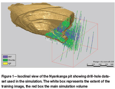
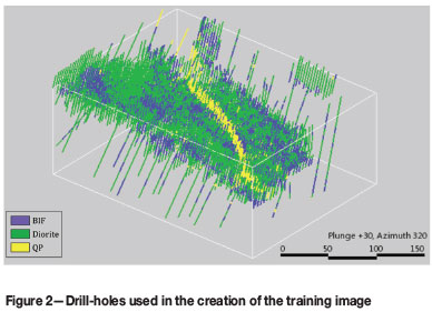
The drill-hole data-set consists of 410 holes, 249 drilled by reverse circulation and 161 by diamond core drilling. The majority of the drill-holes are sampled at 1 m intervals. In the top portion of the deposit, dense grade-control drilling on a grid of 10 m (along easting) by 5 m (along northing) allowed for the definition of a well-informed TI (Figure 2).

 

 

Training image preparation

Choice of a TI for simulation of lithologies is of paramount importance in the application of MPS as it serves as the source of spatial patterns to be simulated.

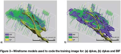
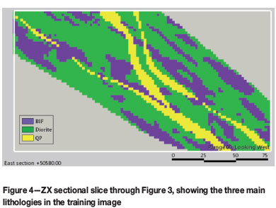
A TI with 742 500 nodes evenly spaced at 2 m intervals was created. Three main lithologies ‒ BIF, intrusive diorite complex, and barren QP dykes ‒ were modelled and used for domaining the gold simulation. The boundary between BIF and diorite was modelled using a radial basis function method. QP dykes were modelled deterministically as tabular bodies. The resulting wireframes were used to code grid nodes in the TI (Figure 3).

 

 

A ZX sectional view of the resulting TI is shown in Figure 4.

 

 

Training image trial simulation

A trial simulation was performed over the volume of the TI to ensure good overall reproducibility of the patterns contained in the image and to confirm the choice of simulation parameters before applying the TI to the main volume of interest.

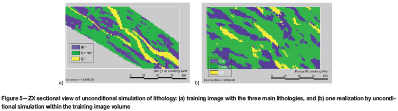
In the unconditional simulation, the connectivity of dykes posed a major challenge, while simulated BIF and diorite shapes were reproduced quite reasonably. A number of parameters were tested, but none of them seemed to improve the connectivity dramatically. A comparison of the TI and the pattern derived by unconditional simulation is given in Figure 5.

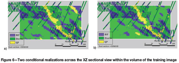
Conditional simulation within the TI volume allowed for better connectivity of dykes, the high density of conditioning data being the main contributing factor. Honouring of the global lithology proportions was good, considering that no global proportions were specified in the simulation input. The comparison is presented in Table I.

 

 

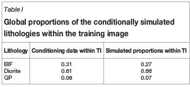
Two realizations of the conditional simulation are displayed in Figure 6a and 6b.

 

 

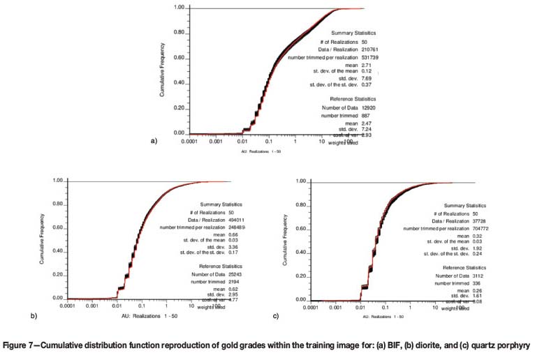
The results of the gold simulation in all three lithology types were compared with the main statistics and gold distributions in the cumulative distribution plots of Figure 7. These diagrams illustrate the extent to which simulated output has honoured the conditioning data.

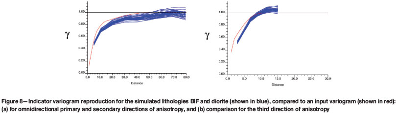
Indicator variograms for the simulated realizations of BIF and diorite lithologies from the TI in the principal directions of continuity (blue) compare well with the input variogram models for both lithologies (red), as shown in Figure 8.

The range and continuity of variograms created from the simulated gold values for each of the three lithologies were compared to the input gold variogram models, which although not perfect matches, were acceptably replicated in the simulation.

Simulation of the orebody

The main simulation for a more extensive volume was done for 50 realizations of both lithology and gold values. The best traditional approach in simulation is to generate 100-200 realizations (Deutsch, 2013) to stabilize the uncertainty and reduce 'uncertainty of the uncertainty' as much as possible. There are too many subjective decisions that might aggravate the uncertainty if a small number of realizations is produced.

The simulation grid consisted of 1 827 360 nodes evenly spaced at 5 m, and covering 470 m easting by 900 m northing by 540 m elevation. In order to reduce the computational demands, a mask object was used to block out the simulation grid nodes away from the mineralized shear zone.

Lithology simulation

Fifty realizations of lithology were performed. The results were subjected to the same tests as in the TI simulation. While reproduction of the BIF and diorite interface did not pose major problems, the issue of poor connectivity of the dykes re-emerged. The effect on the simulated mineral content was considered immaterial in the current case study; however, the issue was pursued to assist in future simulations.

The most satisfactory results were achieved by adding to the simulation input a conditioning grid object and a second TI.

The grid object had nodes flagged as QP if they fell within 20 m distance from the appropriate drill-hole intersections. The outcome of this approach was similar to a combination of hierarchical simulation and locally varying proportions. Figure 9 demonstrates this - the upper part of the simulation grid has higher content of nodes simulated as dykes than the portions down-plunge. This is explained by the higher density of drill coverage in the upper portions of the volume.

 

 

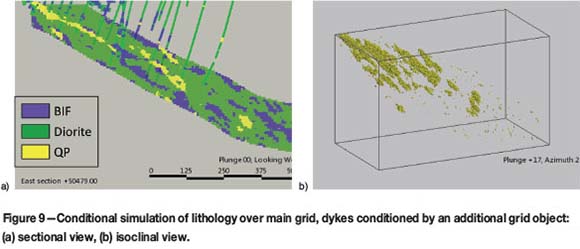
The second TI depicted large-scale repetitive morphology of the dykes, which was not captured in the first TI. Examples of the resulting simulation are shown in Figure 10.

Other DS parameters were tested to improve the continuity of the dykes, such as increasing the number of nodes and radii in the search neighbourhood, and increasing the distance threshold tolerance. None of these resulted in any significant improvement, while imposing higher computational demands.

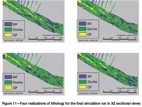
Comparison of four realizations of lithology in the final simulation run in Figure 11 demonstrates the uniqueness of each realization; particularly, the further away it is from the conditioning data.

 

 

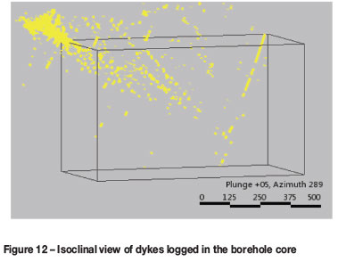
Drill-hole intersections through dykes in 3D display a radial attitude of the intrusions joining down-dip, with a plug-like intrusive body occurring in the top right corner of the simulation grid as seen in Figure 12. The plug-like volume would require defining another stationary domain and yet another TI; no further modelling of this feature is undertaken here. Future simulation work would benefit from the generation of synthetic TIs representing different lithological interfaces (BIF/diorite, host rock/QP dykes) and incorporation of structural readings of lithological contacts from diamond-drill core. Simple synthetic TIs with horizontal attitude of lithological boundaries, combined with a rotational field generated from the structural readings, would allow simulation of a more geologically truthful representation of the reality. Hierarchical simulation with different search parameters for different lithological interfaces would improve the result.

 

 

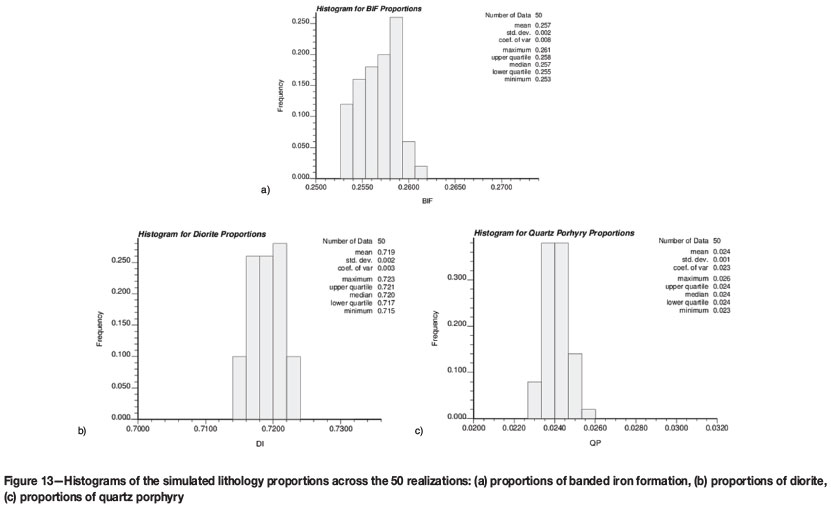
Validation was performed for honouring of lithology proportions. The global lithology proportions used as an additional input for the simulation were determined from the logging information of the conditioning drill-holes. Overall, the average values for the simulated global proportions are maintained. An overall fluctuation of a few per cent was observed across the 50 realizations, as shown in Table II. The effect was considered to be immaterial for the purpose of the study.

 

 

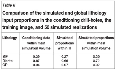
Figure 13 shows the histograms of the simulated proportions, the spread across the realizations being very narrow.

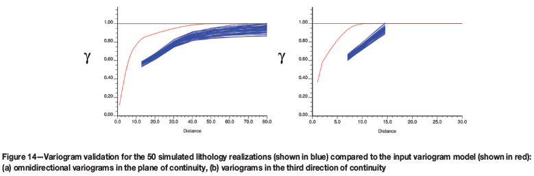
The variogram validation for the interface between the BIF and diorite was done for a portion of the simulation grid in the principal directions of continuity, and is shown in Figure 14. The simulation variograms between the BIF and diorite (blue) produced longer ranges of continuity than the input model (red). Further investigation into the reasons behind this would be beneficial.

A number of DS parameters have been tested to balance the simulation quality and processing time. The algorithm was run in multi-thread mode, using a 64-bit 8-core machine with 2.4 GHz processor. The average time required to produce a single realization of lithology for the main simulation grid was 20 minutes. Recommendations provided in Mariethoz et al. (2012, 2013) were followed to allow reasonable results in minimal time. The final parameters for the lithology simulation, conditioned with 44 780 drill-hole samples, were:

►Consistency of conditioning data: 0.05

►Number of conditioning nodes: 30

►Distance threshold: 0.05

►Distance tolerance for flagging nodes: 0.01

►Maximum fraction of training image to be scanned: 0.3.

Grade simulation

The 50 realizations of lithology were used for subsequent geostatistical domaining in the SGS simulation of 50 realizations for gold grade. Simulations were run for each lithology with the transformation of the gold values into Gaussian space and back being built-in to the SGS algorithm. The Gaussian variogram models based on the densely spaced grade control drilling were supplied as an input to the simulation of grade in each lithological domain.

The realizations of gold grade were validated in the same way as the TI, including visual checking, validation of the statistics, and variogram checking.

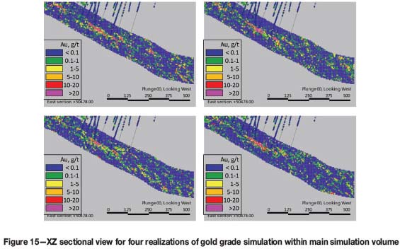
While the drill-hole samples are honoured in each of the realizations, it is also evident that each realization is unique, especially as we move away from the conditioning data. The four realizations in Figure 15 depict the short-range variability inherited from the variogram models of the densely spaced data in the TI. Differences between the realizations represent the joint uncertainty: from the lithology simulation and the grade realizations within it.

 

 

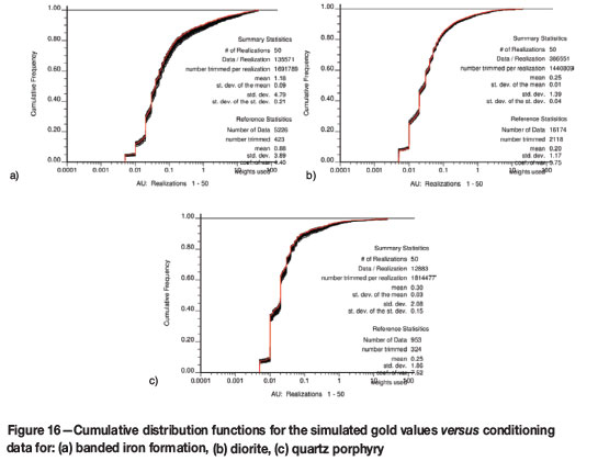
Cumulative distribution functions of gold grades for the simulated realizations and conditioning grades for the different lithology types are compared in Figure 16.

 

 

Gold variogram reproduction was checked within a small portion of the simulation grid, for BIF and diorite lithologies only. The comparison was done for the back-transformed data against the variogram models constructed in the original data units, and is shown in Figure 17 and Figure 18.

 

 

 

 

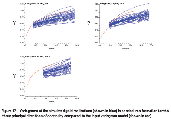
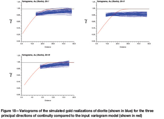
While the gold variograms within the BIF domain display a good fit with the input model, the diorite variograms are not as well-behaved and show a high degree of variance against the original model, as shown in Figure 18.

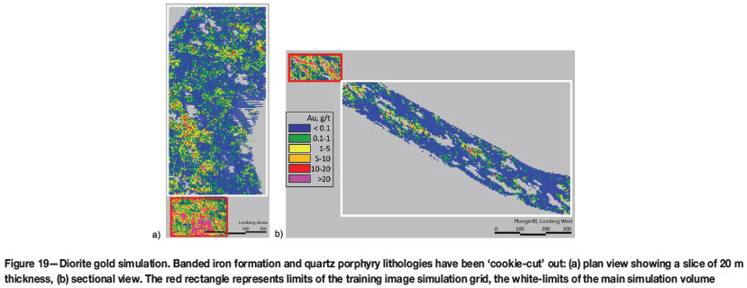
The noise in the variograms of the diorite at a short-scale distance is partially attributed to the fact that the model in the original space reaches 70% of variance within the range of 22-25 m for the main continuity plane. This distance, expressed in terms of the simulation grid nodes, represents separation of 2-3 nodes as the orientation of anisotropy is oblique to the geometry of the simulation grid, the smallest lag separation distance being about 7.5 m. An example realization of gold within diorite in Figure 19 shows sporadic mineralization down the plunge of the orebody. Another explanation is that insufficient care has been taken in deciding on the extents of the volume for variogram validation. The volume spanned the shear zone boundary and contained samples of high- and low-grade stationary domains, thereby introducing additional noise into the variograms. It would be beneficial to run the variogram validation in Gaussian space. A simulation grid of finer resolution should be used to allow reproduction of short-scale continuity.

 

Analysing uncertainty

The geostatistical processing necessary for assimilating and interpreting the simulation outputs requires that the uncertainty be summarized to represent a joint uncertainty between lithology and grade. A number of options for summarizing both the lithology and grade realizations using GSLIB software (Deutsch and Journel, 1998) exist; the emphasis here is given to assessing uncertainty at a local level rather than on a global scale.

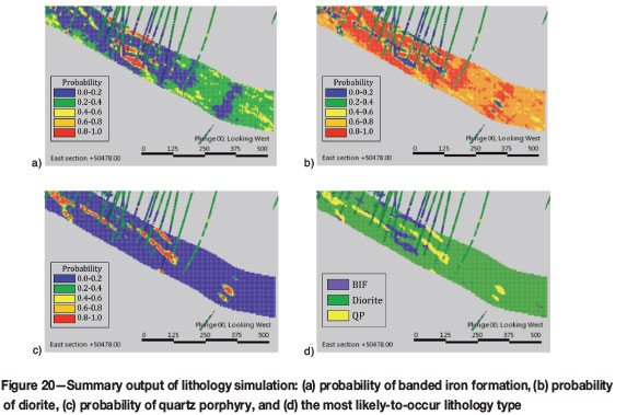
The weighted average summary of 50 realizations of the lithology created as an output a grid object with the probability of each lithology type, a most-likely-to-occur lithology and entropy, examples of which are shown in Figure 20. Post-processing for the most-likely-to-occur lithology would be similar to the results arising from indicator kriging.

 

 

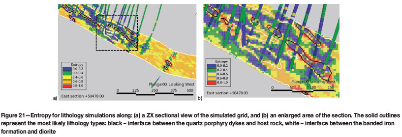
The concept of entropy was propounded as far back as 1933 (Pauli, 1933; Shannon, 1948), and was introduced to geostatistics by Christakos in 1990. In the context of geosta-tistics, it is simply described as 'gain in knowledge'. Lower entropy values are observed in well-informed areas, where conditional probabilities are determined with high confidence. An example of this is shown in the cross-section of the orebody in Figure 21a and in the enlarged inset in Figure 21b. The highest entropy occurs along the peripheries of the most likely dykes, as this is the lithology with the highest uncertainty in the study.

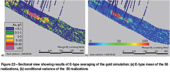
The cross-sectional views of the conditional variance of the simulated gold values and the expected mean for 50 realizations are shown in Figure 22. Strong dependency or so-called 'proportional effect' between the local mean and the conditional variance is observed; a common feature in positively skewed distributions. It expresses itself as high-grade areas having greater variability, and hence greater uncertainty, than low-grade areas. For lognormal distributions, the local standard deviation is proportional to the local mean (Journel and Huijbregts, 1978).

 

 

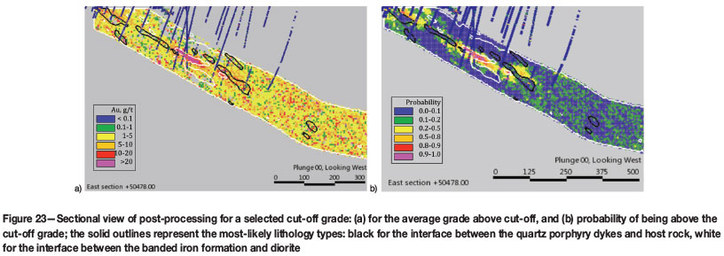
The results of post-processing for a specific grade cut-off are shown in Figure 23, together with the outlines of the wireframes representing the most likely lithology, for ease of interpretation.

The tendency for high-grade values to be smeared across the simulation volume in the absence of conditioning data (Figure 23a and 23b) reflects a need to improve stationarity domaining. This had a material effect on the uncertainty assessment in the study. For future work, high-grade zones along the shear should be placed in a separate domain.

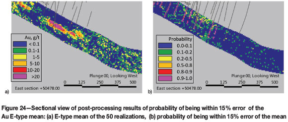
An example of post-processing for a specified probability interval to be within a relative error of the mean is shown in Figure 24. The short-scale variogram ranges induce a probability of 90% being observed in the vicinity of the drillholes.

 

 

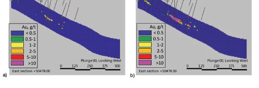
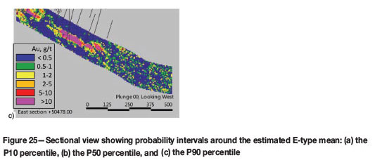
Different percentiles of probability intervals around the estimated E-type mean are displayed in Figure 25. The P10 percentile (Figure 25a) and P90 percentile (Figure 25c) are the symmetric 80% probability intervals around the E-type mean. The areas that are most certainly high in relation to the mean are shown as high-grade areas on the lower limit P10 percentile map. On the P90 percentile map, low grades are indicative of areas that are most certainly low grade. The P50 percentile map (Figure 25b) represents the most likely outcome.

 

 

Block averaging to recoverable resources

High-resolution simulation grids cannot be used efficiently. The advantage of simulating into a fine-resolution grid is that an upscaling to a different SMU size is possible, providing consistency of results. If the cell support is fine enough in comparison with the variogram model ranges, volume-variance relationships can be bypassed. Fine-resolution realizations upscaled to panel-size support can be used for further processing in the mine planning process; upscaling to SMU-size support can be used to assess uncertainty in the mine scheduling process.

For continuous variables involved in the estimation of the mineral resources, such as mineral concentrations and densities of rock types, averaging to a larger support size is linear. This means that for continuous variables the mean stays constant within the volume being upscaled. For categorical variables, the most probable lithology is assigned to larger size blocks by volume weighting.

Smoothing in the variables and uncertainty takes place during upscaling. This effect can be seen in Figure 26, which shows the fine-resolution simulation of 5 m nodes spacing (Figure 26a and 26b) and a version upscaled to a node spacing of 40 m easting x 40 m northing x 10 m elevation (Figure 26c and 26d). Large variability observed at a small scale is considerably smoothed in large-scale cells. Upscaled realizations can be processed to generate grade-tonnage curves that provide a representation of uncertainty in the recoverable metal.

The mining optimization should be performed for all upscaled realizations. It can also be done for a few selected realizations, which can be chosen based on different transfer functions or performance calculations (Deutsch, 2013), such as metal content or degree of 'connectivity' between panel blocks above a chosen cut-off grade. In this case, the scenarios could be a P50 percentile, which would represent a base case, with the P10 and P90 percentiles providing 80% confidence limits.

 

Discussion

In the current study, the MPS simulation approach for generating realizations of mineralized units has been combined with a traditional SGS simulation of grade. The Direct Sampling multi-point algorithm employed in the lithology simulation proved to be fast and flexible. Many parameters are available to ensure good reproduction of the patterns found in the training image, and good connectivity while maintaining global proportions of lithologies. Difficulties were encountered when simulating dykes. In terms of final uncertainty assessment, reproducing the continuity of dykes was of negligible importance; it was pursued in order to improve our understanding of the algorithm and for more effective use in future. Using an additional TI depicting large-scale morphology of dykes combined with distance-based conditioning for the grid nodes in the vicinity of the drill-holes, although not a holistically ideal approach, produced the most significant improvement. Implementing hierarchical simulation in the algorithm, as well as different search parameters for different lithological interfaces, would ease the task in future.

In the current case study, a traditional parametric algorithm such as sequential indicator simulation would have probably yielded sufficiently good and similar results for simulation of the BIF and diorite lithologies. It would, however, have failed at reproducing the morphology of dykes.

The possibility of running DS in multi-core mode makes it competitive with many other commercially available algorithms. This paper applies DS to a simple project, but the method can be implemented to more complex cases where variograms cannot be used to describe the continuity or to validate results.

The validation of the gold simulation results produced poorly-behaved variograms within the diorite domain. Probable reasons are insufficient resolution of the simulation grid to capture the short-scale variability, and non-stationarity.

Some practical considerations to be born in mind when performing simulation:

► Start with non-conditioned simulation until the pattern reproduction is good. The insufficiencies in parameters will come through in the main simulation where conditioning data is sparser

►Test parameters and keep track of both processing time and the quality of reproduction using a common reference location for easier comparison

►Full-scale features, such as boudin-like compartmentalizing of the host rock by dykes, must be present in the TI with sufficient repetition to avoid the effect of 'patching'

►Statistics for both continuous and categorical variables must be thoroughly checked in the early stages of simulation to enable reasonableness of the applied parameters and appropriate stationarity decisions to be validated

►Using trend as an additonal input into the SGS would assist in dealing with non-stationarity

►Performing a simulation exercise using exploration drill-holes only, within a production area, can allow reconciliation analysis to back-up the simulation results

►As anisotropy is borrowed from the TI, there will be short-scale continuity in the realizations and the simulation results might present noise

►Structural features logged in diamond-drill core could be used to impose better control on simulated geological boundaries

►Particular care needs to be taken when choosing a TI. It is the TI that carries the decision on stationarity and geological settings to be simulated over the entire volume of interest. The best approach is to have a stationary generic TI, and deal with any non-stationarity by the means of 'soft' conditioning: trends, local proportions, and potential fields for use on rotation and homothety.

The examples of uncertainty assessments demonstrate the value of information provided by stochastic simulations. The stochastic approach and uncertainty assessment are model-dependent and stationarity-dependent, and must rely on a robust quantitative validation of the model. Analysing the data and geological settings to make an appropriate decision on stationarity is crucial if statements about uncertainty are to be valid. Improper decisions about stationarity, as has been unintentionally demonstrated in the current study, result in higher uncertainty.

Realizations can be processed through a transfer function or performance calculation. In the context of mining it may be a grade-tonnage curve, the degree of connectivity between the ore/waste blocks, or mine scheduling. Realizations may be ranked in order to select a few for detailed processing.

The value of the stochastic approach to modelling is that it provides an appreciation of the extent of uncertainty when making an appropriate decision. On the other hand, it is also possible to average outcomes of many realizations and produce a smoothed result which is very close to that obtained by kriging.

Quantitative uncertainty, e.g. probability of being within ±15% with 90% confidence, can be used to support geometric criteria for classifying reserves and resources. In this way, probabilistic meaning will enhance classification and make it easier to understand for a non-specialist.

Uncertainty assessment is often not intuitive. Gold mineralization, for example, is characterized by skewed distributions and the proportional effect. This increased variability in the extreme values increases and spreads the uncertainty response, while larger proportions of low values tend to be associated with low uncertainty. Spatial correlation is relevant, since poor spatial correlation causes increase in uncertainty, and vice versa.

Stochastic modelling, and an MPS method in particular, increases the amount of technical work and computing power required. However, acceptance or rejection of a TI is more visual than a parametric model. It can be more inviting for involvement of specialist geological expertise, besides geostatisticians, and would provide more integration of different skills and ownership for field geologists.

 

References

Brayshaw, M., Nugus, M., and Robins, S. 2010. Reassessment of controls on the gold mineralisation in the Nyankanga deposit ‒ Geita Gold Mines, Northwestern Tanzania. 8th International Mining Geology Conference, Queenstown, New Zealand, 21-24 August 2011. Australasian Institute of Mining and Metallurgy. pp. 153-168.         [ Links ]

Caers, J. 2011 Modelling Uncertainty in the Earth Sciences. Wiley-Blackwell, Chichester, UK. pp. 90-106.         [ Links ]

Christakos, G. 1990. A Bayesian/maximum-entropy view to the spatial estimation problem. Mathematical Geology, vol. 22, no. 7. pp. 763-777.         [ Links ]

Deutsch, C. and Journel, A. 1998. GSLIB: Geostatistical Software Library and User's Guide. 2nd edn. Oxford University Press, Oxford.         [ Links ]

Deutsch, C. 2013. Lectures on Citation Program in Applied Geostatistics, presented in Johannesburg, RSA. Centre for Computational Geostatistics. University of Alberta, Edmonton, Alberta, Canada.         [ Links ]

Goovaerts, P. 1997. Geostatistics for Natural Resource Evaluation. Oxford University Press, New York.         [ Links ]

Guardiano, F. and Srivastava, R. 1993. Multivariate geostatistics: beyond bivariate moments. Quantitative Geology and Geostatistics, vol. 5. pp. 133-144.         [ Links ]

Honarkhah, M. and Caers, J. 2010 Stochastic simulation of patterns using distance-based pattern modelling. Mathematical Geosciences, vol. 42, no. 5. pp. 487-517.         [ Links ]

Journel, A. and Huijbregts, C. 1978. Mining Geostatistics. Academic Press, p. 187.         [ Links ]

Mariethoz, G., Meerschman, E., Pirot, G., Straubhaar, J., Van Meirvenne, M., and Renard, P. 2012. Guidelines to perform multiple-point statistical simulations with the Direct Sampling algorithm. Ninth International Geostatistics Congress, Oslo, Norway, 11-15 June 2012.         [ Links ]

Mariethoz, G., Meerschman, E., Pirot, G., Straubhaar, J., Van Meirvenne, M., and Renard, P. 2013. A practical guide to performing multiple-point statistical simulations with the Direct Sampling algorithm. Computers and Geosciences, vol. 52. pp. 307-324.         [ Links ]

Pauli, W. 1933. Die allgemeinen Prinzipien der Wellenmechanik. Handbuch der Physik. Geiger, H. and Scheel,K. (eds.). Springer, Berlin. 2nd edn, vol. 24, part 1 . pp. 83-272.         [ Links ]

Perez, C. and Ortiz, J. 2011. Mine-scale modeling of lithologies with multipoint geostatistical simulation. IAMG, 2011, University of Salzburg, 5-9 September 2011 . pp. 123-132.         [ Links ]

Remy, N., Boucher, A., and Wu, J. 2009. Applied Geostatistics with SGeMS.. Cambridge University Press.         [ Links ]

Rezaee, H., Mariethoz, G., Koneshloo, M., and Asghari, O. 2013. Multiple-point geostatistical simulation using the bunch-pasting Direct Sampling method. Computers and Geosciences, vol. 54. pp. 293-308.         [ Links ]

Shannon, C. 1948 A mathematical theory of communication. Bell System Technical Journal, vol. 27. pp. 379-423, 623-656.         [ Links ]

Straubhaar, J., Renard, P., Mariethoz, G., Froidevaux, R., and Besson, O. 2011. An improved parallel multiple-point algorithm using a list approach. Mathematical Geosciences, vol. 43. pp. 305-328.         [ Links ]

Tahmasebi, P., Hezarkhani, A., and Sahimi, M. 2012. Multiple-point geostatistical modelling based on the cross-correlation functions. Computational Geosciences, vol. 16, no. 3. pp. 779-797.         [ Links ]

Wu, J., Boucher, A., and Zhang, T. 2008. A SGeMS code for pattern simulation of continuous and categorical variables: FILTERSIM. Computers and Geosciences, vol. 34, no. 12. pp. 1863-1876.         [ Links ]

Zhang, T., Switzer, P., and Journel, A. 2006. Filter based classification of training image patterns for spatial simulation. Mathematical Geology, vol. 38, no. 1. pp. 63-80.         [ Links ]