DANIE KRIGE COMMEMORATIVE EDITION - VOLUME III

 

Regression revisited (again)

 

 

I. Clark

Geostokos Limited, Scotland

 

 

---

SYNOPSIS

One of the seminal pioneering papers in reserve evaluation was published by Danie Krige in 1951. In that paper he introduced the concept of regression techniques in providing better estimates for stope grades and correcting for what later became known as the 'conditional bias'. In South Africa, the development of this approach led to the phenomenon being dubbed the 'regression effect', and regression techniques ultimately formed the basis of simple kriging in Krige's later papers. In the late 1950s and early 1960s, Georges Matheron (1965) formulated the general theory of 'regionalized variables' and included copious discussion on what he termed the 'volume-variance' effect. Matheron defined mathematically the reason for, and quantification of, the difference in variability between estimated values and the actual unknown values. In 1983, this author published a paper that combined these two philosophies so that the 'regression effect' could be quantified before actual mining block values were available. In 1996 and in some earlier presentations, Krige revisited the regression effect in terms of the conditional bias and suggested two measures that might enable a practitioner of geostatistics to assess the 'efficiency' of the kriging estimator in any particular case. In this article, we revisit the trail from 'regression effect' to 'kriging efficiency' in conceptual terms and endeavour to explain exactly what is measured by these parameters and how to use (or abuse) them in practical cases.

Keywords: geostatistics, block estimation, regression effect, conditional bias, kriging efficiency.

---

 

 

Introduction

In recent years, major mining and geostatistical software packages have included additional parameters in block kriging analyses, such as a 'regression' coefficient and a measure of 'kriging efficiency'. Krige (1996) presented a paper at the APCOM conference in Wollongong discussing factors that affect these parameters during resource estimation. These measures were discussed by Snowden (2001) in her section dealing with classification guidelines released by the AusIMM.

While 'kriging efficiency' is a relatively new concept, the 'regression effect' has been in use in southern Africa for over 60 years. In this paper, the basis and development of the regression parameter will be explained in detail and illustrated with an uncomplicated case study. This illustration shows that while a regression correction might correct for the 'conditional bias', it does not necessarily improve the confidence in the estimated value for an individual mining block. The relevance of 'kriging efficiency' in the assessment of confidence in estimated block values, and a simple discriminator between indicated and inferred values, are also discussed.

The aim of this paper is to show that modern practice world-wide is well founded on over a half-century of established practice in southern Africa, pioneered by Krige on the gold mines, by illustration with a simulated example where the geology is continuous and homogeneous, and precise and accurate sampling is carried out on a square grid with grades that are normally distributed.

 

The case study

The full database of sampling is as close to exhaustive as possible (less than 0.5% of the range of influence). A block size typical for mine planning and grade control is used throughout this paper, although other (larger) block sizes were studied. This block size corresponds to around 10% of the full range of influence on the semivariogram. Around 700 blocks are available for assessment and analysis.

The exhaustive sampling is combined to provide 'actual block averages' from the 625 sample points that lie within each of the blocks in this model. The simplest estimation method - ordinary kriging (OK) - is used throughout this discussion, although similar estimation results could probably be obtained using inverse distance squared.

 

Varying the sample density

Sampling grids were studied at grid sizes varying from centre of every block (10% of the range of influence) up to centre of every sixth block (60% of the range of influence). For simplicity, we present results here only from grids at three and six times the block size. Expressed another way, the two sampling grids correspond to 30% and 60% of the range of influence respectively.

 

Quantifying the regression effect

Krige's original discussions (1951) were based on very large data-sets available from Witwatersrand-type gold reefs where chip samples were taken initially in development drives and then, as mining proceeded, on each stope face advance. The average grade of the development samples was used to evaluate the likely average of a stope panel of (say) 30 m by 30 m. As the stoping panel was mined out, face samples were used to evaluate the next advance into the stope. As a result, once the stope is mined out, a dense grid of samples is available to determine what was actually mined from that stope.

Krige found that, even allowing for the lognormal nature of the gold values, there was a discrepancy between the average stope value and the average development value. A simple scatter plot of development versus stope averages showed that the relationship between them is neither perfect nor clustered around the 45° line.

In 1972, this author was asked to look into the same question for Geevor Tin Mines Limited in Cornwall, UK. Again, the question was why development averages did not match the stope values found during mining. Again, the obvious approach was to plot development against stope averages to find out where the discrepancy arose.

In this paper we illustrate the approach with a simple example that could be considered as a single bench through an open pit, with drilling on a square grid used to estimate the values within each planned mining block.

 

Sparse sampling - sampling grid spacing six blocks

OK using an isotropic semivariogram model and search radius at the full range of influence was applied to produce a block model for this illustration. The block size is realistic at 10% of the range of influence, and sampling is relatively sparse at six times the block size. Around 700 blocks were estimated.

A scattergram of the actual block average along the vertical axis and ordinary kriged estimates along the horizontal axis is shown in Figure 1. The 'perfect estimator' is shown as a dashed line with a slope of 1 on this graph. It can be seen clearly that the points on the graph do not lie around this 45° line. The estimated values have a much smaller spread or 'dispersion' around the centre of the graph than do the actual values.

 

 

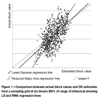
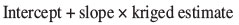
In classical statistics, a 'best fit' line can be fitted through the points to find the slope of the line that 'best' fits the points. In least squares regression (LS), the 'best' line (solid line in Figure 1) is that which minimizes the difference between the true average block value and the value that would be estimated using the regression line. This slope is calculated by:

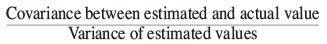
and the intercept on the line is determined by making sure that the line passes through the average value of all the points for each variable. According to stated theory, application of these regression factors to the estimates produces a new estimate of the form:

which should 'correct' for the regression effect and produce estimates that lie around the 45° line. However the scattergram of the kriged estimate corrected for the regression effect using the LS approach shown in Figure 2 shows little difference from Figure 1.

 

 

Other types of regression

There are other types of regression lines that can be used to 'correct' the estimated values. One of these is the 'reduced major axis' (RMA) form, which calculates the slope as:

(cf. Till, 1974). This slope simply rescales the estimates to have the same dispersion as the true values. This is a highly simplified version of an 'affine correction'. Figure 1 shows the RMA regression as a dotted line, and Figure 3 shows a plot of the corrected estimates using RMA versus the actual block averages. This scatter lies more pleasingly around the 45° line.

 

 

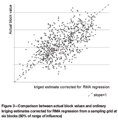
It should, perhaps, be noted that the confidence on individual corrected estimates will not be affected by the correction if (and only if) the actual average value over the study area is exactly known. The intercept on the regression line requires the knowledge of the actual block values. In this illustration the true average value is known for every block and for the whole area. This should be borne in mind for the further sections of this paper.

 

Deriving the regression parameter without historical mining data

In Krige's early work and in the illustration here, the database contains enough information to evaluate the 'actual' values that are being estimated. Witwatersrand-type gold has been mined since the 19th century and copious amounts of sampling data were available for a study such as this. In this author's early studies, around 50 stopes had already been mined before the correction factors were developed. With the advent of Matheron's theory of regionalized variables (1965) it became apparent that the regression parameters could be determined before half the deposit had been mined out.

Matheron showed that the semivariogram model - under certain assumptions − was mathematically equivalent to calculating the covariance model. That is, the covariance between two values a certain distance apart can be found from:

This relationship can also be used to derive dispersion variances for blocks, viz:

In fact, the covariance between any two sets of entities -samples or blocks - can be derived from the semivariogram model for the samples. The development of the mathematics for the regression factors can be found in Clark (1983).

Krige (1996) uses the following notation:

►BV represents the dispersion variance of block values within the deposit or study area

►KV represents the kriging variance obtained during the estimation of the block.

In more traditional geostatistical notation:

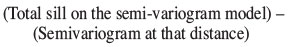
►BV = total sill on the semivariogram

►

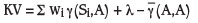
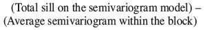
where the total sill on the semivariogram is taken to be the best estimate for the dispersion variance of single samples within the study area. (A,A) represents the average semivariogram within the block, also known as the 'within block variance'. γ(S_i,A) is the semivariogram between each sample and the block being estimated, and wi represents the weight given to that sample.

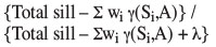
For each block in the model, the slope of the relevant LS regression line can be calculated as follows:

where λ represents the Lagrangian multiplier produced in the solution of the OK equations when using the semivariogram form. If the OK equations are solved using covariances instead of semivariograms, the sign should be reversed on the Lagrangian multiplier. In Snowden's (2001) notation, μ = -λ.

Note that this formula is not actually quoted in Krige (1996). In more traditional geostatistical notation, this formula (cf. Clark 1983) would be written:

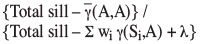
To calculate the RMA slope for each block, the formula becomes:

Note also that the formula in Snowden (2001) uses the absolute value of μ. This would be correct if μ is negative, but not if μ is positive (i.e. λis negative). It is possible for the λ value to be negative if the sampling layout is very dense or (at least) excessive to needs.

All of the parameters needed to generate the regression slope are available during the OK process, so that the calculation of the regression slope demands very little extra computation time during block estimation. In this way, the regression slope appropriate to each individual block estimate can be evaluated and included in the output for the block kriging exercise. In Figures 2, 3, and 4 the individual regression parameters were used to provide the 'corrected' estimate in each case.

 

 

Kriging efficiency

The major parameter proposed in Krige (1996) and documented in Snowden (2001) is the 'kriging efficiency'. This is a comparative measure of confidence in the individual block estimate. In Krige's (1996) notation, this parameter is calculated as:

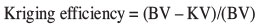
and is usually expressed as a percentage rather than the proportion that would be given by the formula. Figure 5 shows the relationship between LS and RMA parameters and the kriging efficiency to the kriging variance for each block, using the sparse data grid.

 

 

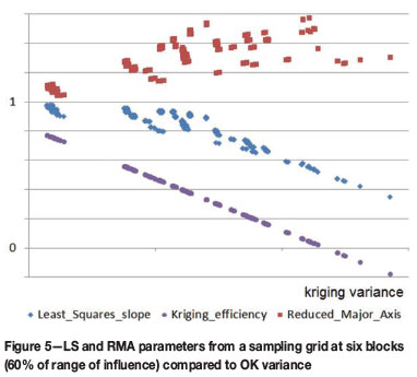
It should be noted that kriging efficiency can take a negative value. As discussed in Krige (1996), the situation for which KV = BV is when the kriging estimate provides the same level of reliability as simply using the global average value as the block estimate. This author coined the term ygiagam¹ for this phenomenon and uses this criterion to indicate when resources or reserves should be classified as Inferred. As a general rule, any block with negative kriging efficiency should never be included in a Measured resource category. The sampling grid chosen for this illustration - 60% of the range of influence of the semivariogram - equates very approximately to the spacing at which kriging efficiency tends to zero. It is also close to the distance which many practitioners use for 'Measured' resources.

 

Denser sampling grid

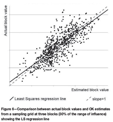
As a (possibly) more realistic exercise, a sampling grid at three-block spacing was also studied. Figure 6 shows the kriged estimates versus the actual block values, the 45° line, and the overall regression slope for the (almost) 700 blocks.

 

 

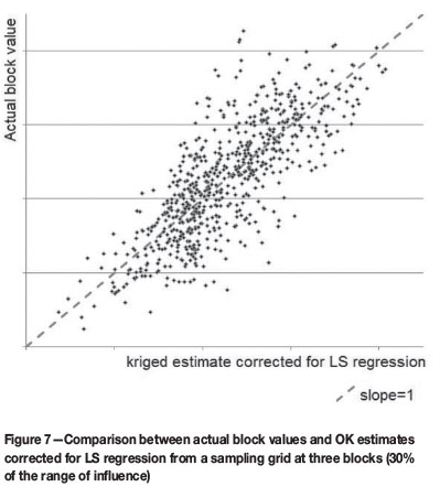
The closer sampling interval (three blocks) brings actual and kriged estimates corrected by the LS regression coefficient into much closer agreement, as shown in Figure 7.

 

 

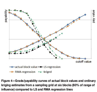
Effect on the grade/payability curve

The effect of data spacing on the estimated block values is evident in the grade/payability curves of actual block values from sampling grids of different sizes. Figure 8 compares two restricted data-sets at three block and six block spacing with the exhaustive potential data-set. This graph indicates that more widely spaced sampling is unlikely to fully represent the high or low values that could be encountered during mining. According to this example, the limited data-sets give a similar general behaviour as regards value (pay grade) but seriously underestimate the likely payable tonnage.

 

 

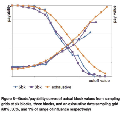
Figure 9 compares the kriged block estimates based on the two sample spacings with the actual block values. The sparse data seriously over-estimates the payability for low grades and under-estimates the payability for higher cut-offs - as would be expected by the smoothing shown in previous sections. The grade estimated by kriging the six-block sparse grid seriously underestimates the recovered grade at any cutoff compared to the actual block values.

 

 

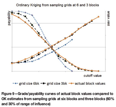
In contrast, the closer spaced sampling (three times block size) is almost identical to the pay grades in the actual blocks for every cut-off, but it seems to over-estimate payability at low cut-offs. A similar graph using the RMA corrected block grades for the six-block sampling and the LS corrected block grades from the three-block sampling would show almost identical grade/payability curves in this particular case.

 

Misclassification of ore and waste

The studies reported in this paper, in Clark (1983), and in Krige (1951, 1996) all illustrate how consideration of the regression effect - or conditional bias - can improve estimates for a mining block or stoping model. It is apparent, however, that emphasis on the potentially marginal improvements achieved by regression correction has masked a far more important consideration in mine planning based on estimated block models. Whatever the regression coefficient or the kriging efficiency, there still remains the fact that values allocated to potential mining blocks are still only estimates.

For any particular cut-off value, there will be blocks that are estimated as payable which will actually be waste. There will be blocks that are estimated to be below cut-off which will actually be payable. This problem is also discussed in detail in Krige's early work (1951) and many later papers. Figure 10 illustrates the problem of applying cut-off values to the estimated block values using our example with the three-block sampling, where the regression effect is minimal.

 

 

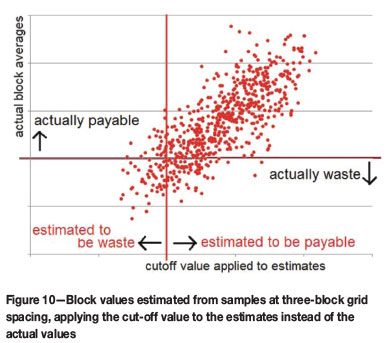
The majority of estimated block values are classified correctly as payable or waste. However, a significant number of blocks are misclassified. The practical implication of this is that blocks that are actually payable on average will be sent to the waste pile (or not mined), while waste material will be mined and delivered to the plant as payable. However much mathematics is applied to this situation, the result will be the same tonnage mined for a lower overall recovered value.

It should be emphasized that this is not a result of using a particular estimation technique, but is a fact of production. The only way to eliminate this effect is to instigate a grade control sampling plan that will narrow the scatter on the graph enough to achieve an absolute minimum of blocks in the two punitive quadrants. Or, in simpler language, to achieve a good enough grade control programme to be fully confident in the block values during production.

As a final illustration, a single cut-off was applied to the block estimates using the three-block sampling for OK. Those blocks estimated as above cut-off were separated from those classified as 'waste'. Grade/payability curves were produced from these two sets of blocks and are shown in Figure 11.

 

 

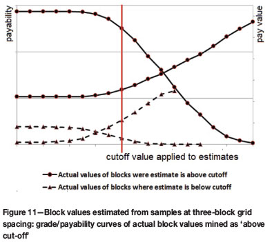
In this case, the payability curves are scaled to reflect how many blocks are classified as payable as opposed to waste. This example illustrates the proportion of 'payable' blocks that are actually non-payable and the values in the blocks that are classified as 'waste'.

 

Conclusions

Most of the above illustrations could equally well have been produced using theoretical methods. It is not necessary to have a vast database of previously mined areas to produce the regression factors or an assessment of the likely misclas-sification errors that will be incurred during production. This paper has used a case study where the database is exhaustive because it has been created from a conditional simulation based on a real-life case study.

It should be borne in mind that regression corrections, kriging efficiency, and misclassification assessments depend heavily on the sample values following a normal(-ish) behaviour. Statistics such as variance and covariance have little real meaning when applied to skewed sample data.

The example presented shows that least squares regression works well when the regression slope is less than (or not much greater than) 1. If a high degree of smoothing is present, an alternative approach such as RMA regression or affine corrections should be utilized, rather than least squares. Alternatively, simulation studies may be valuable when data is too sparse to achieve realistic results.

It cannot be emphasized strongly enough that a regression correction does not improve confidence in individual estimated block values. There will always be uncertainty in the true value of the block until it has been mined (and maybe afterwards). Misclassification of payable and non-payable blocks will inevitably lead to reconciliation problems during production - unless allowances are built into the mine plan for those recovery factors.

One puzzling factor is that many software packages now supply regression factors but do not seem to use them in adjusting the block estimates.

Kriging efficiency is simply a standardized form of the kriging variance. An advantage over simply considering the kriging variance is that it does provide an immediate indication of the ygiagam guideline as to where to stop trying to provide a local estimate for an individual block.

The main aim of this paper has been to show that approaches developed by Danie Krige 60 years ago are still vital in the production of mineral resource and reserve models and in ongoing mine planning.

 

References

Clark, I. 1983. Regression revisited. Mathematical Geology, vol. 15, no. 4. pp. 517-536.         [ Links ]

Krige, D.G. 1951. A statistical approach to some basic mine valuation problems on the Witwatersrand. Journal of the Chemical, Metallurgical and Mining Society of South Africa, vol. 52. pp. 119-139.         [ Links ]

Krige, D.G. 1996. A practical analysis of the effects of spatial structure and of data available and accessed, on conditional biases in ordinary kriging. 5th International Geostatistics Congress, Wollongong, Australia 22-27 September 1996. Vol. 2. Baafi, E.Y. and Schofield, N.A. (eds.). Springer. pp. 799-810.         [ Links ]

Matheron, G. 1965. La Theorie des Variables Regionalisees et ses Applications. Masson, Paris.         [ Links ]

Snowden, D.V. 2001. Practical interpretation of mineral resource and ore reserve classification guidelines. Mineral Resource and Ore Reserve Estimation - The AusIMM Guide to Good Practice. Edwards. A.C. (ed.). Monograph 23. Australasian Intitute of Mining and Metallurgy, Melbourne. pp. 643-652.         [ Links ]

TILL, R. 1974. Statistical Methods for the Earth Scientist. Palgrave MacMillan. 168 pp.         [ Links ]

 

 

1 Your guess is as good as mine’