DANIE KRIGE COMMEMORATIVE EDITION - VOLUME III

 

Dealing with high-grade data in resource estimation

 

 

O. Leuangthong^I; M. Nowak^II

^ISRK Consulting (Canada) Inc., Toronto, ON, Canada
^IISRK Consulting (Canada) Inc., Vancouver, BC, Canada

 

 

---

SYNOPSIS

The impact of high-grade data on resource estimation has been a longstanding topic of interest in the mining industry. Concerns related to possible over-estimation of resources in such cases have led many investigators to develop possible solutions to limit the influence of high-grade data. It is interesting to note that the risk associated with including high-grade data in estimation appears to be one of the most broadly appreciated concepts understood by the general public, and not only professionals in the resource modelling sector. Many consider grade capping or cutting as the primary approach to dealing with high-grade data; however, other methods and potentially better solutions have been proposed for different stages throughout the resource modelling workflow.
This paper reviews the various methods that geomodellers have used to mitigate the impact of high-grade data on resource estimation. In particular, the methods are organized into three categories depending on the stage of the estimation workflow when they may be invoked: (1) domain determination; (2) grade capping; and (3) estimation methods and implementation. It will be emphasized in this paper that any treatment of high-grade data should not lead to undue lowering of the estimated grades, and that limiting the influence of high grades by grade capping should be considered as a last resort. A much better approach is related to domain design or invoking a proper estimation methodology. An example data-set from a gold deposit in Ontario, Canada is used to illustrate the impact of controlling high-grade data in each phase of a study. We note that the case study is by no means comprehensive; it is used to illustrate the place of each method and the manner in which it is possible to mitigate the impact of high-grade data at various stages in resource estimation.

Keywords: grade domaining, capping, cutting, restricted kriging.

---

 

 

Introduction

A mineral deposit is defined as a concentration of material in or on the Earth's crust that is of possible economic interest. This generic definition is generally consistent across international reporting guidelines, including the South African Code for Reporting of Exploration Results, Mineral Resources and Mineral Reserves (SAMREC Code), Canadian Securities Administrators' National Instrument 43-101 (NI 43-101), and the Australasian Code for Reporting of Exploration Results, Mineral Resources and Ore Reserves (2012), published by the Joint Ore Reserves Committee (the JORC Code). Relative to its surroundings, we can consider that a mineral deposit is itself an outlier, as it is characterized by an anomalously high concentration of some mineral and/or metal. This presents an obvious potential for economic benefit, and in general, the higher the concentration of mineral and/or metal, the greater the potential for financial gain.

Indeed, many mining exploration and development companies, particularly junior companies, will publicly announce borehole drilling results, especially when high-grade intervals are intersected. This may generate public and/or private investor interest that may be used for project financing. Yet, it is interesting that these high-grade intercepts that spell promise for a mineral deposit present a challenge to resource modellers in the determination of a resource that will adequately describe ultimately unknown in-situ tons and grade.

Resource estimation in the mining industry is sometimes considered an arcane art, using old methodologies. It relies on well-established estimation methods that have seen few advancements in the actual technology used, and it is heavily dependent on the tradecraft developed over decades of application. Unlike in other resource sectors, drilling data is often readily available due to the accessibility of prospective projects and the affordability of sample collection. As such, the 'cost' of information is often low and the relative abundance of data translates to reduced uncertainty about the project's geology and resource quality and quantity. It is in this context that more advanced geostatistical developments, such as conditional simulation (see Chiles and Delfiner (2012) for a good summary of the methods) and multiple point geostatistics (Guardiano and Srivastava, 1992; Strebelle and Journel, 2000; Strebelle, 2002), have struggled to gain a stronghold as practical tools for mineral resource evaluation.

So we are left with limited number of estimation methods that are the accepted industry standards for resource modelling. However, grade estimation is fundamentally a synonym for grade averaging, and in this instance, it is an averaging of mineral/metal grades in a spatial context. Averaging necessarily means that available data is accounted for by a weighting scheme. This, in itself, is not an issue nor is it normally a problem, unless extreme values are encountered. This paper focuses on extreme high values, though similar issues may arise for extreme low values, particularly if deleterious minerals or metals are to be modelled. High-grade intercepts are problematic if they receive (1) too much weight and lead to a possible over-estimation, or if kriging is the method of choice, (2) a negative weight, which may lead to an unrealistic negative estimate (Sinclair and Blackwell, 2002). A further problem that is posed by extreme values lies in the inference of first-and second-order statistics, such as the mean, variance, and the variogram for grade continuity assessment. Krige and Magri (1982) showed that presence of extreme values may mask continuity structures in the variogram.

This is not a new problem. It has received much attention from geologists, geostatisticians, mining engineers, financiers, and investors from both the public and private sectors. It continues to draw attention across a broad spectrum of media ranging from discussion forums hosted by professional organizations (e.g. as recently as in 2012 by the Toronto Geologic Discussion Group) and online professional network sites (e.g. LinkedIn.com). Over the last 50 years, many geologists and geostatisticians have devised solutions to deal with these potential problems arising from high-grade samples.

This paper reviews the various methods that geomodellers have used or proposed to mitigate the impact of high-grade data on resource estimation. In particular, the methods are organized into three categories depending on the stage of the estimation workflow when they may be invoked: (1) domain determination; (2) grade capping; and (3) estimation methods and implementation. Each of these stages is reviewed, and the various approaches are discussed. It should be stressed that dealing with the impact of high-grade data should not lead to undue lowering of estimated grades. Very often it is the high-grade data that underpins the economic viability of a project.

Two examples are presented, using data from gold deposits in South America and West Africa, to illustrate the impact of controlling high-grade data in different phases of a study. We note that the review and examples are by no means comprehensive; they are presented to illustrate the place of each method and the manner in which it is possible to mitigate the impact of high-grade data at various stages in resource estimation.

 

What constitutes a problematic high-grade sample?

Let us first identify which high-grade sample(s) may be problematic. Interestingly, this is also the section where the word outlier is normally associated with a 'problematic' high-grade sample. The term outlier has been generally defined by various authors (Hawkins, 1980; Barnett and Lewis, 1994; Johnson and Wichern, 2007) as an observation that deviates from other observations in the same grouping. Many researchers have also documented methods to identify outliers.

Parker (1991) suggested the use of a cumulative coefficient of variation (CV), after ordering the data in descending order. The quantile at which there is a pronounced increase in the CV is the quantile at which the grade distribution is separated into a lower grade, well-behaved distribution and a higher grade, outlier-influenced distribution. He proposes an estimation of these two parts of the distribution, which will be discussed in the third stage of dealing with high-grade data in this manuscript.

Srivastava (2001) outlined a procedure to identify an outlier, including the use of simple statistical tools such as probability plots, scatter plots, and spatial visualization, and to determine whether an outlier can be discarded from a database. The context of these guidelines was for environmental remediation; however, these practical steps are applicable to virtually any resource sector.

The identification of spatial outliers, wherein the local neighbourhood of samples is considered, is also an area of much research. Cerioli and Riani (1999) suggested a forward search algorithm that identifies masked multiple outliers in a spatial context, and provides a spatial ordering of the data to facilitate graphical displays to detect spatial outliers. Using census data for the USA, Lu et al. (2003, 2004) have documented and proposed various algorithms for spatial outlier detection, including the mean, median, and iterative r (ratio) and iterative z algorithms. Liu et al. (2010) devised an approach for large, irregularly spaced data-sets using a locally adaptive and robust statistical analysis approach to detect multiple outliers for GIS applications.

In general, many authors agree that the first task in dealing with extreme values is to determine the validity of the data, that is, to confirm that the assay values are free of errors related to sample preparation, handling, and measurement. If the sample is found to be erroneous, then the drill core interval should be re-sampled or the sample should be removed from the assay database. Representativeness of the sample selection may also be confirmed if the interval is re-sampled; this is particularly relevant to coarse gold and diamond projects. If the sample is deemed to be free of errors (excluding inherent sample error), then it should remain in the resource database and subsequent treatment of this data may be warranted.

 

Stages of high-grade treatment

Once all suspicious high-grade samples are examined and deemed to be correct, such that they remain part of the resource database, we now concern ourselves with how this data should be treated in subsequent modelling. For this, we consider that there are three particular phases of the resource workflow wherein the impact of high-grade samples can be explicitly addressed. Specifically, these three stages are:

1. Domaining to constrain the spatial impact of high grade samples

2. Grade capping or cutting to reduce the values of high-grade samples

3. Restricting the spatial influence of high-grade samples during estimation.

The first stage of domaining addresses the stationarity of the data-set, and whether geological and/or grade domaining can assist in properly grouping the grade samples into some reasonable grouping of data. This may dampen the degree by which the sample(s) is considered high; perhaps, relative to similarly high-grade samples, any one sample appears as part of this population and is no longer considered an anomaly.

The second phase is that which many resource modellers consider a necessary part of the workflow: grade capping or cutting. This is not necessarily so; in fact, some geostatis-ticians are adamant that capping should never be done, that it represents a 'band-aid' solution and masks the real problem, which is likely linked to stationarity decisions and/or an unsuitable estimation method.

The third phase, where the influence of a high-grade sample may be contained, is during the actual estimation phase. In general, this can occur in one of two ways: (1) as an implementation option that may be available in some commercial general mining packages (GMPs); or (2) a non-conventional estimation approach is considered that focuses on controlling the impact of high-grade samples.

The following sections discuss the various approaches that may be considered in each of these three stages of addressing high-grade samples. We note that these three stages of treating high grades are not necessarily mutually exclusive. For instance, grade domaining into a higher grade zone does not pre-empt the use of grade capping prior to resource estimation. In fact, most mineral resource models employ at least one or some combination of the three stages in resource evaluation.

Stage 1: Domaining high-grade data

Resource modelling almost always begins with geological modelling or domaining. This initial stage of the model focuses on developing a comprehensive geological and structural interpretation that accounts for the available drillhole information and an understanding of the local geology and the structural influence on grade distribution. It is common to generate a three-dimensional model of this interpretation, which is then used to facilitate resource estimation. In many instances, these geological domains may be used directly to constrain grade estimation to only those geological units that may be mineralized.

It is also quite common during this first stage of the modelling process to design grade domains to further control the distribution of grades during resource estimation. One of the objectives of grade domaining is to prevent smearing of high grades into low-grade regions and vice versa. The definition of these domains should be based on an understanding of grade continuity and the recognition that the continuity of low-grade intervals may differ from that of higher grade intervals (Guibal, 2001; Stegman, 2001).

Often, a visual display of the database should help determine if a high-grade sample comprises part of a subdomain within the larger, encompassing geological domain. If subdomain(s) can be inferred, then the extreme value may be reasonable within the context of that subpopu-lation.

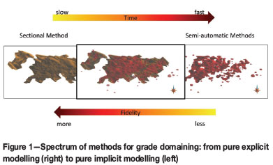
Grade domains may be constructed via a spectrum of approaches, ranging from the more time-consuming sectional method to the fast, semi-automatic boundary or volume function modelling methods (Figure 1). The difference between these two extremes has also been termed explicit versus implicit modelling, respectively (Cowan et al., 2002; 2003; 2011). Of course, with today's technology, the former approach is no longer truly 'manual' but commonly involves the use of some commercial general mine planning package to generate a series of sections, upon which polylines are digitized to delineate the grade domain. These digitized polylines are then linked from section to section, and a 3D triangulated surface can then be generated. This process can still take weeks, but allows the geologist to have the most control on interpretation. The other end of the spectrum involves the use of a fast boundary modelling approach that is based on the use of radial basis functions (RBFs) to create isograde surfaces (Carr et al., 2001, Cowan et al., 2002; 2003; 2011). RBF methods, along with other linear approaches, are sensitive to extreme values during grade shell generation, and often some nonlinear transform may be required. With commercial software such as Leapfrog, it can take as little as a few hours to create grade shells. In between these two extremes, Leuangthong and Srivastava (2012) suggested an alternate approach that uses multigaussian kriging to generate isoprobability shells corresponding to different grade thresholds. This permits uncertainty assessment in the grade shell that may be used as a grade domain.

 

 

In practice, it is quite common that some semi-automatic approach and a manual approach are used in series to generate reasonable grade domains. A boundary modelling method is first applied to quickly generate grade shells, which are then imported into the manual wireframing approach and used, in conjunction with the projected drill-hole data, to guide the digitization of grade domains.

Stegman (2001) used case studies from Australian gold deposits to demonstrate the importance of grade domains, and highlights several practical problems with the definition of these domains, including incorrect direction of grade continuity, too broad (or tight) domains, and inconsistency in data included/excluded from domain envelopes. Emery and Ortiz (2005) highlighted two primary concerns related to grade domains: (1) the implicit uncertainty in the domain definition and associated boundaries, and (2) that spatial dependency between adjacent domains is unaccounted for. They proposed a stochastic approach to model the grade domains and the use of cokriging of data across domains to estimate grades.

Stage 2: Capping high-grade samples

In the event that grade domaining is not viable and/or insufficient to control the influence of one or more high-grade samples, then more explicit action may be warranted in order to achieve a realistic resource estimate. In these instances, grade capping or cutting to some level is a common practice in mineral resource modelling. This procedure is also sometimes referred to as 'top cut', 'balancing cut', or a 'cutting value'. It generally involves reducing those grade values that are deemed to be outliers or extreme erratic values to some lower grade for the purposes of resource evaluation. Note that this practice should never involve deletion of the high-grade sample(s) from the database.

Two primary reasons for capping high-grade samples are: (1) there is suspicion that uncapped grades may overstate the true average grade of a deposit; and (2) there is potential to overestimate block grades in the vicinity of these high-grade samples. Whyte (2012) presented a regulator's perspective on grade capping in mineral resource evaluation, and suggested that the prevention of overestimation is good motivation to consider grade capping. For these reasons, capping has become a 'better-safe-than-sorry' practice in the mining industry, and grade capping is done on almost all mineral resource models (Nowak et al., 2013).

Given the prevalence of this approach in mining, it is no surprise that there are a multitude of tools available to help a modeller determine what grade value is an appropriate threshold to cap. These include, but are not limited to, the use of probability plots, decile analysis (Parrish, 1997), metal-at-risk analysis, cutting curves (Roscoe, 1996), and cutting statistics plots. Nowak et al. (2013) compared four of these approaches in an application to a West African gold deposit (Figure 2).

 

 

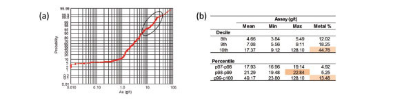
Probability plots are likely the most commonly used tool, due to their simplicity and the availability of software to perform this type of analysis. Inflection points and/or gaps in the distribution are often targeted as possible capping values (Figure 2a). In some instances, legacy practice at a particular mine site may dictate that capping is performed at some threshold, e.g. the 95th percentile of the distribution. In these cases, the initial decision to cap at the 95th percentile may well have been reasonable and defensible; however, this choice should be revisited and reviewed every time the database and/or domains are updated.

Parrish (1997) introduced decile analysis, which assesses the metal content within deciles of the assay distribution. Total metal content for each decile and percentage of the overall metal content are calculated. Parrish suggested that if the top decile contains more than 40% of the metal, or if it contains more than twice the metal content of the 80% to 90% decile, then capping may be warranted (Figure 2b). Analysis then proceeds to split the top decile into percentiles. If the highest percentiles have more than 10% of the total metal content, a capping threshold is chosen. The threshold is selected by reducing all assays from the high metal content percentiles to the percentile below which the metal content does not exceed 10% of the total.

The metal-at-risk procedure, developed by H. Parker and presented in some NI 43-101 technical reports, e.g. (Neff et al., 2012), uses a method based on Monte Carlo simulation. The objective of the process is to establish the amount of metal which is at risk, i.e., potentially not present in a domain for which resources will be estimated. The procedure assumes that the high-grade data can occur anywhere in space, i.e., there is no preferential location of the high-grade data in a studied domain. The assay distribution can be sampled at random a number of times with a number of drawn samples representing roughly one year's production. For each set of drawn assays a metal content represented by high-grade composites can be calculated. The process is repeated many times, and the 20th percentile of the high-grade metal content is applied as the risk-adjusted amount of metal. Any additional metal is removed from the estimation process either by capping or by restriction of the high-grade assays.

Cutting curves (Roscoe, 1996) were introduced as a means to assess the sensitivity of the average grade to the capped grade threshold. The premise is that the average grade should stabilize at some plateau. The cap value should be chosen as near the inflection point prior to the plateau (Figure 2c), and should be based on a minimum of 500 to 1000 samples.

Cutting statistics plots, developed by R.M. Srivastava and presented in some internal technical reports for a mining company in the early 1990s, consider the degradation in the spatial correlation of the grades at various thresholds using an indicator approach (personal communication, 1994). The capping values are chosen by establishing a correlation between indicators of assays in the same drill-holes via downhole variograms, at different grade thresholds. Assays are capped at the threshold for which correlation approaches zero (Figure 2d).

Across the four approaches illustrated in Figure 2, the proposed capping value ranges from approximately 15 g/t to 20 g/t gold, depending on the method. While the final selection is often in the hands of the Qualified Person, a value in this proposed range can generally be supported and confirmed by these multiple methods. In any case, the chosen cap value should ensure a balance between the loss in metal and loss in tonnage.

Stage 3: Estimating with high-grade data

Once we have 'stabilized' the average grade from assay data, we can now focus further on how spatial location of very high-grade assays, potentially already capped, affects estimated block grades. The risk of overstating estimated block grades is particularly relevant in small domains with fewer assay values and/or where only a small number of data points are used in the estimation. The first step in reviewing estimated block grades is to visually assess, on section or in plan view, the impact of high-grade composites on the surrounding block grades. Swath plots may also be useful to assess any 'smearing' of high grades. This commonly applied, simple, and effective approach is part of the good practice recommended in best-practice guidelines, and can be supplemented by additional statistical analysis. The statistical analysis may be particularly useful if a project is large with many estimation domains.

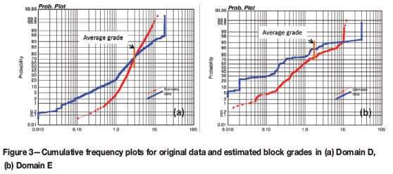
One simple way to test for potential of overestimation in local areas could be a comparison of cumulative frequency plots from data and from estimated block grades. Let us consider two domains, a larger Domain D, and amuch smaller Domain E, both with positively skewed distributions which are typically encountered in precious metal deposits. A typical case, presented in Figure 3(a) for Domain D, shows that for thresholds higher than average grade, the proportion of estimated block grades above the thresholds is lower than the proportion of high-grade data. This is a typical result from smoothing the estimates. On the other hand, in Domain E, we see that the proportion of high-grade blocks above the overall average is higher than the proportion from the data (Figure 3b). We can consider this as a warning sign that those unusual results could potentially be influenced by very high-grade assays that have undue effect on the overall estimates.

 

 

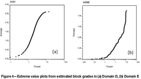
Cutting curve plots can be also quite helpful; however, in this instance we are not focused on identifying a capping threshold, but rather the impact of high-grade blocks on the overall average block grade. Figure 4 shows the average estimated block grades below a set of thresholds in domains D and E. In Domain D (Figure 4a) there is a gradual increase in average grades for increasing thresholds, eventually stabilizing at 2. 7 g/t Au. On the other hand, in Domain E (Figure 4b) there is a very abrupt increase in average grade for very similar high-grade block estimates. This indicates a relatively large area(s) with block estimates higher than 6 g/t.

 

 

Limiting spatial influence of high-grade samples

If the result of these early estimation validation steps reveals that high-grade composites may be causing over-estimation of the resource, then we may wish to consider alternative implementation options in the estimation that may be available within software. Currently, a few commercial general mining packages offer the option to restrict the influence of high-grade samples. That influence is specified by the design of a search ellipsoid with dimensions smaller than that applied for grade estimation.

Typically the choice of the high-grade search ellipsoid dimensions is based on an educated guess. This is based on a notion that the size of the high-grade search ellipsoid should not extent beyond the high-grade continuity. There are, however, two approaches that the authors are aware of that are potentially better ways to assess high-grade continuity.

The first approach involves assessing the grade continuity via indicator variograms. The modeller simply calculates the indicator variograms for various grade thresholds. As the focus is on the high-grade samples, the grade thresholds should correspond to higher quantiles, likely above the 75th percentile. A visual comparison of the indicator variograms at these different thresholds may reveal a grade threshold above which the indicator variogram noticeably degrades. This may be a reasonable threshold to choose to determine which samples will be spatially restricted. The range of the indicator variogram at that threshold can also be used to determine appropriate search radii to limit higher grade samples.

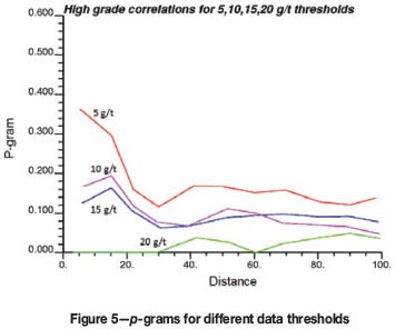
The second approach is also quantitative, and relies on a p-gram analysis developed by R.M. Srivastava (personal communication, 2004). The p-gram was developed in the petroleum industry to optimize spacing for production wells. To construct p-grams, assay composites are coded with an indicator at a threshold for high-grade population. Using a process similar to that for indicator variography, the data is paired over a series of lag distances. Unlike the conventional variogram, the p-gram considers only the paired data in which the tail of the pairs is above the high-grade threshold. The actual p-gram value is then calculated as the ratio of pairs where both the head and tail are above the threshold to the number of pairs where the tail of the pair is above the threshold. Pairs at shorter lag distances are given more emphasis by applying an inverse distance weighting scheme to the lag distance. Figure 5 shows an example of a p-gram analysis for a series of high-grade thresholds. The curves represent average probability that two samples separated by a particular distance will both be above the threshold, given that one is already above the threshold. In this specific example, up to a threshold of 15 g/t gold, the range of continuity, i.e., the distance at which the curve levels off, is 30 m. This distance can be applied as search ellipsoid radius to limit high-grade assays.

 

 

Alternative estimation approaches for high-grade mitigation

While the above methods work within the confines of a traditional estimation framework for resource estimation, there are alternative, lesser known estimation methods that were proposed specifically to deal with controlling the influence of high-grade samples. Journel and Arik (1988) proposed an indicator approach to dealing with outliers, wherein the high grade falls within the last class of indicators and the mean of this class is calculated as the arithmetic average of samples in the class. Parker (1991) pointed out that using the arithmetic average for this last class of indicators may be inefficient or inaccurate. Instead, Parker (1991) proposed a procedure that first identifies which threshold should be chosen to separate the high grades from the rest of the sample population (discussed earlier), and secondly proposes an estimation method that combines an indicator probability and the fitting of a lognormal model to the samples above the threshold to calculate the average grade for this class of data, . A block grade is then obtained by combining estimates of both the lower and higher grade portions of the sample data: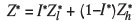, where the superscript^* denotes an estimate, I^* is the probability of occurrence of lower grades below the threshold, and is the kriged estimate of the block using only those samples below the threshold. The implicit assumption is that there is no correlation between the probability and grade estimates.

Arik (1992) proposed a two-step kriging approach called 'outlier restricted kriging' (ORK). The first step consists of assigning to each block at location X the probability or the proportion Φ(Χ, Z_c) of the high-grade data above a predefined cut-off Z_c. Arik determines this probability based on indicator kriging at cut-off grade Z_c. The second step involves the assignment of the weights to data within a search ellipsoid. These weights are assigned in such a way that the sum of the weights for the high-grade data is equal to the assigned probability Φ(χ, Z_c) from the first step. The weights for the other data are constrained to add up to 1 -Φ(Χ, Z_c). This is similar to Parker's approach in the fact that indicator probabilities are used to differentiate the weights that should be assigned to higher grade samples and lower grade samples.

Costa (2003) revisited the use of a method called robust kriging (RoK), which had been introduced earlier by Hawkins and Cressie (1984). Costa showed the practical implementation of RoK for resource estimation in presence of outliers of highly skewed distributions, particularly if an erroneous sample value was accepted as part of the assay database. It is interesting to note that where all other approaches discussed previously were concerned with the weighting of higher grade samples, RoK focuses on directly editing the sample value based on how different it is from its neighbours. The degree of change of a sample value is controlled by a user-specified c parameter and the kriging standard deviation obtained from kriging at that data location using only the surrounding data. For samples that are clearly part of the population, i.e. not considered an outlier or an extreme value, then the original value is left unchanged. For samples that fall within the extreme tail of the grade distribution, RoK yields an edited value that brings that sample value closer to the centre of the grade distribution.

More recently, Rivoirard et al. (2012) proposed a mathematical framework called the top-cut model, wherein the estimated grade is decomposed into three parts: a truncated grade estimated using samples below the top-cut grade, a weighted indicator above the top-cut grade, and an independent residual component. They demonstrated the application of this top-cut model to blast-hole data from a gold deposit and also to a synthetic example.

 

Impact of various treatments - examples

Two examples are presented to illustrate the impact of high-grade samples on grade estimation, and the impact of the various approaches to dealing with high-grade data. In both cases, data from real gold deposits is used to illustrate the results from different treatments.

Example 1: West African gold deposit

This example compares the estimation of gold grades from a West African gold deposit. Three different estimations were considered: (1) ordinary kriging with uncapped data; (2) ordinary kriging with capped data; and (3) Arik's ORK method with uncapped data. Table I shows an example of estimated block grades and percentage of block grades above a series of cut-offs in a mineralized domain from this deposit. At no cut-off, the average estimated grade from capped data (2.0 g/t) is almost identical to the average estimated grades from the ORK method (2.04 g/t). On the other hand, the coefficient of variation CV is much higher from the ORK method, indicating much higher estimated block grade variability. This result is most likely closer to actually recoverable resources than the over-smoothed estimates from ordinary kriging. Once we apply a cut-off to the estimated block grades, the ORK method returns a higher grade and fewer recoverable tons, which is in line with typical results during mining when either blast-hole or underground channel samples are available.

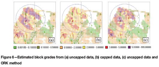
It is interesting to note that locally the estimated block grades can be quite different. Figure 6 shows the estimated high-grade area obtained from the three estimation methods. Not surprisingly, ordinary kriging estimates from uncapped data result in a relatively large area with estimated block grades higher than 3 g/t (Figure 6a). Capping results in the absence of estimated block grades higher than 5 g/t (Figure 6b). On the other hand, estimation from uncapped data with the ORK method results in block estimated grades located somewhere between the potentially too-optimistic (uncapped) and too-pessimistic (capped) ordinary kriged estimates (Figure 6c).

 

 

Example 2: South American gold deposit

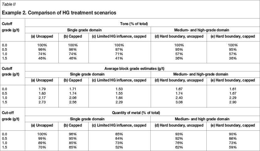
This second example compares five different approaches to grade estimation on one primary mineralized domain from a South American gold deposit. This one domain is considered to generally be medium grade; however, an interior, continuous high-grade domain was identified, modelled, and considered for resource estimation.

The first three methods consider a single grade domain, while the last two cases consist of two grade domains: the initial medium-grade shell with an interior high-grade shell. Therefore, the last two cases make use of grade domaining as another means to control high-grade influence. Specifically, the five cases considered for comparison are:

(a) One grade domain, uncapped composites

(b) One grade domain, capped composites

(c) One grade domain, capped composites with limited radii imposed on higher grade values

(d) Two grade domains, uncapped data with a hard boundary

(e) Two grade domains, capped data with a hard boundary.

In all cases, estimation is performed using ordinary kriging. Case (a) is referred to as the base case and is effectively a do-nothing scenario. Case (b) considers only the application of grade capping to control high-grade influence. Case (c) considers a two-phase treatment of high-grade data, namely capping grades and also limiting the influence of those that are still considered to be high-grade samples but remain below the cap value. The limiting radii and threshold were chosen based on a preliminary assessment of indicator variograms for various grade thresholds. The last two cases introduce Phase 1 treatment via domaining as another possible solution, with uncapped and capped composites, respectively.

Table II shows a comparison of the relative tons for this mineralized domain as a percentage of the total tons, the average grade of the block estimates, and the relative metal content shown as a percentage of the total ounces relative to the base case, at various cut-off grades. At no cut-off and when only a single grade domain is considered (i.e. cases (a) to (c)), we see that capping has only a 4% impact in reducing the average grade and consequently ounces, while limiting the influence of high grade with capping reduces the average grade and ounces by 15%. Results from cases (d) to (e) show that the impact of the grade domain is somewhere between that of using capped data and limiting the influence of the high-grade data. At cut-off grades of 1.0 g/t gold and higher, cases (d) and (e) show a significant drop in tonnage accompanied by much higher grades than the single domain case. In ounces, however, the high-grade domain yields global results similar to the high-grade limited radii option.

To compare the local distribution of grades, a cross-section is chosen to visualize the different cases considered (Figure 7). Notice the magnified region in which a composite gold grade of 44.98 g/t is found surrounded by much lower gold grades. Figures 7a to 7c correspond to the single grade domain, while Figures 7d and 7e correspond to high-grade treatment via domaining, where the interior high-grade domain is shown as a thin polyline. From the base case (Figure 7a), it is easy to see that this single high-grade sample results in a string of estimated block grades higher than 3 g/t. Using capped samples (Figure 7b) has minimal impact on the number of higher grade blocks. Interestingly, limiting the high-grade influence (Figure 7c) has a similar impact to high-grade domaining (Figures 7d and 7e) in that same region. However, the high-grade domain definition has a larger impact on the upper limb of that same domain, where a single block is estimated at 3 g/t or higher, with the majority of the blocks surrounding the high-grade domain showing grades below 1 g/t.

In this particular example, the main issue lies in the overarching influence of some high-grade composites. Capping accounted for a reduction of the mean grade of approximately 7%; however, it is the local impact of the high grade that is of primary concern. A high-grade domain with generally good continuity was reliably inferred. As such, this more controlled, explicit delineation of a high-grade region is preferred over the more dynamic approach of limiting high-grade influence.

 

Discussion

Many practitioners, geologists, and (geo) statisticians have tackled the impact of high-grade data from many perspectives, broadly ranging from revisiting stationarity decisions to proposals of a mathematical framework to simple, practical tools. The list of methods to deal with high-grade samples in resource estimation in this manuscript is by no means complete. It is a long list, full of good sound ideas that, sadly, many in the industry have likely never heard of. We believe this is due primarily to a combination of software inaccessibility, professional training, and/or time allocated to project tasks.

There remains the long-standing challenging of making these decisions early in pre-production projects, where an element of arbitrariness and/or wariness is almost always present. The goal should be to ensure that the overall contained metal should not be unreasonably lost. Lack of data in early stage projects, however, makes this judgement of representativeness of the data challenging. For later stage projects where production data is available, reconciliation against production should be used to guide these decisions.

This review is intended to remind practitioners and technically-minded investors alike that mitigating the influence of high-grade data is not fully addressed simply by top-cutting or grade capping. For any one deposit, the challenges of dealing with high-grade data may begin with an effort to 'mine' the different methods presented herein and/or lead to other sources whereby a better solution is found that is both appropriate and defensible for that particular project.

 

Conclusions

It is interesting to note the reaction when high-grade intercepts are discovered during drilling. On the one hand, these high-grade intercepts generate excitement and buzz in the company and potentially the business community if they are publicly announced. This is contrasted with the reaction of the geologist or engineer who is tasked with resource evaluation. He or she generally recognizes that these same intercepts pose challenges in obtaining reliable and accurate resource estimates, including potential overestimation, variogram inference problems, and/or negative estimates if kriging is the method of estimation. Some mitigating measure(s) must be considered during resource evaluation, otherwise the model is likely to be heavily scrutinized for being too optimistic. As such, the relatively straightforward task of top-cutting or grade capping is almost a de facto step in constructing most resource models, so much so that many consider it a 'better safe than sorry' task.

This paper reviews different approaches to mitigate the impact of high-grade data on resource evaluation that are applicable at various stages of the resource modelling workflow. In particular, three primary phases are considered: (1) domain design, (2) statistical analysis and application of grade capping, and/or (3) grade estimation. In each stage, various methods and/or tools are discussed for decision-making. Furthermore, applying a tool/method during one phase of the workflow does not preclude the use of other methods in the other two phases of the workflow.

In general, resource evaluation will benefit from an understanding of the controls of high-grade continuity within a geologic framework. Two practical examples are used to illustrate the global and local impact of treating high-grade samples. The conclusion from both examples is that a review of any method must consider both a quantitative and qualitative assessment of the impact of high-grade data prior to acceptance of a resource estimate from any one approach.

 

Acknowledgments

The authors wish to thank Camila Passos for her assistance with preparation of the examples.

 

References

Arik, A. 1992. Outlier restricted kriging: a new kriging algorithm for handling of outlier high grade data in ore reserve estimation. Proceedings of the 23rd International Symposium on the Application of Computers and Operations Research in the Minerals Industry. Kim, Y.C. (ed.). Society of Mining Engineers, Littleton, CO. pp. 181-187.         [ Links ]

Barnett, V. and Lewis, T. 1994. Outliers in Statistical Data. 3rd edn. John Wiley, Chichester, UK.         [ Links ]

Carr, J.C., Beaton, R.K., Cherrie, J.B., Mitchell, T.J., Fright, W.R., McCallum, B.C., and Evans, T.R. 2001. Reconstruction and representation of 3D objects with radial basis function. SIGGRAPH '01 Proceedings of the 28th Annual Conference on Computer Graphics and Interactive Techniques, Los Angeles, CA, 12-17 August 2001. Association for Computing Machinery, New York. pp. 67-76.         [ Links ]

Cerioli, A. and Riani, M. 1999. The ordering of spatial data and the detection of multiple outliers. Journal of Computational and Graphical Statistics, vol. 8, no. 2. pp. 239-258.         [ Links ]

Chiles, J.P. and Delfiner, P. 2012. Geostatistics - Modeling Spatial Uncertainty. 2nd edn. Wiley, New York.         [ Links ]

Costa, J.F. 2003. Reducing the impact of outliers in ore reserves estimation. Mathematical Geology, vol. 35, no. 3. pp. 323-345.         [ Links ]

Cowan, E.J., Beatson, R.K., Fright, W.R., McLennan, T.J., and Mitchell, T.J. 2002. Rapid geological modelling. Extended abstract: International Symposium on Applied Structural Geology for Mineral Exploration and Mining, Kalgoorlie, Western Australia, 23-25 September 2002. 9 pp.         [ Links ]

Cowan, E.J., Beatson, R.K., Ross, H.J., Fright, W.R., McLennan, T.J., Evans, T.R., Carr, J.C., Lane, R.G., Bright, D.V., Gillman, A.J., Oshust, P.A., and Titley, M. 2003. Practical implicit geological modelling. 5th International Mining Geology Conference, Bendigo, Victoria, November 17-19, 2003. Dominy, S. (ed.). Australasian Institute of Mining and Metallurgy Melbourne. Publication Series no. 8. pp. 89-99.         [ Links ]

Cowan, E.J., Spragg, K.J., and Everitt, M.R. 2011. Wireframe-free geological modelling - an oxymoron or a value proposition? Eighth International Mining Geology Conference, Queenstown, New Zealand, 22-24 August 2011. Australasian Institute of Mining and Metallurgy, Melbourne. pp 247-260.         [ Links ]

Emery, X. and Ortiz, J.M. 2005. Estimation of mineral resources using grade domains: critical analysis and a suggested methodology. Journal of the South African Institute of Mining and Metallurgy, vol. 105. pp. 247-256.         [ Links ]

Guardiano, F. and Srivastava, R.M. 1993. Multivariate geostatistics: beyond bivariate moments. Geostatistics Troia, vol. 1. Soares, A. (ed.). Kluwer Academic, Dordrecht. pp. 133-144.         [ Links ]

Guibal, D. 2001. Variography - a tool for the resource geologist. Mineral Resource and Ore Reserve Estimation - The AusIMM Guide to Good Practice. Edwards, A.C. (ed.). Australasian Institute of Mining and Metallurgy, Melbourne.         [ Links ]

Hawkins, D.M. 1980. Identification of Outliers. Chapman and Hall, London.         [ Links ]

Hawkins, D.M. and Cressie, N. 1984. Robust kriging - a proposal. Mathematical Geology, vol. 16, no. 1. pp. 3-17.         [ Links ]

Johnson, R.A. and Wichern, D.W. 2007. Applied Multivariate Statistical Analysis, 6th edn. Prentice-Hall, New Jersey.         [ Links ]

Journel, A.G. and Arik, A. 1988. Dealing with outlier high grade data in precious metals deposits. Proceedings of the First Canadian Conference on Computer Applications in the Mineral Industry, 7-9 March 1988. Fytas, K., Collins, J.L., and Singhal, R.K. (eds.). Balkema, Rotterdam. pp. 45-72.         [ Links ]

Krige, D.G. and Magri, E.J. 1982. Studies of the effects of outliers and data transformation on variogram estimates for a base metal and a gold ore body. Mathematical Geology, vol. 14, no. 6. pp. 557-564.         [ Links ]

Leuangthong, O. and Srivastava, R.M. 2012. On the use of multigaussian kriging for grade domaining in mineral resource characterization. Geostats 2012. Proceedings of the 9th International Geostatistics Congress, Oslo, Norway, 10-15 June 2012. 14 pp.         [ Links ]

Liu, H., Jezek, K.C., and O'Kelly, M.E. 2001. Detecting outliers in irregularly distributed spatial data sets by locally adaptive and robust statistical analysis and GIS. International Journal of Geographical Information Science, vol. 15, no. 8. pp 721-741.         [ Links ]

Lu, C.T., Chen, D., and Kou, Y. 2003. Algorithms for spatial outlier detection. Proceedings of the Third IEEE International Conference on Data Mining (ICDM '03), Melbourne, Florida, 19-22 November 2003. DOI 0-7695-1978-4/03. 4 pp.         [ Links ]

Lu, C.T., Chen, D., and Kou, Y. 2004. Multivariate spatial outlier detection. International Journal on Artificial Intelligence Tools, vol. 13, no. 4. pp 801-811.         [ Links ]

Neff, D.H., Drielick, T.L., Orbock, E.J.C., and Hertel, M. 2012. Morelos Gold Project: Guajes and El Limon Open Pit Deposits Updated Mineral Resource Statement Form 43-101F1 Technical Report, Guerrero, Mexico, June 18 2012. http://www.torexgold.com/i/pdf/reports/Morelos-NI-43-101-Resource-Statement_Rev0_COMPLETE.pdf 164 pp.         [ Links ]

Nowak, M., Leuangthong, O., and Srivastava, R.M. 2013. Suggestions for good capping practices from historical literature. Proceedings of the 23rd World Mining Congress 2013, Montreal, Canada, 11-15 August 2013. Canadian Institute of Mining, Metallurgy and Petroleum. 10 pp.         [ Links ]

Parker, H.M. 1991. Statistical treatment of outlier data in epithermal gold deposit reserve estimation. Mathematical Geology, vol. 23, no. 2. pp 175-199.         [ Links ]

Parrish, I.S. 1997. Geologist's Gordian knot: to cut or not to cut. Mining Engineering, vol. 49. pp 45-49.         [ Links ]

Rivoirard, J., Demange, C., Freulon, X., Lecureuil, A., and Bellot, N. 2012. A top-cut model for deposits with heavy-tailed grade distribution. Mathematical Geosciences, vol. 45, no. 8. pp. 967-982.         [ Links ]

Roscoe, W.E. 1996. Cutting curves for grade estimation and grade control in gold mines. 98th Annual General Meeting, Canadian institute of Mining, Metallurgy and Petroleum, Edmonton, Alberta, 29 April 1996. 8 pp.         [ Links ]

Sinclair, A.J. and Blackwell, G.H. 2002. Applied Mineral Inventory Estimation.Cambridge University Press, Cambridge.         [ Links ]

Srivastava, R.M. 2001. Outliers - A guide for data analysts and interpreters on how to evaluate unexpected high values. Contaminated Sites Statistical Applications Guidance Document no. 12-8, British Columbia, Canada. 4 pp. http://www.env.gov.bc.ca/epd/remediation/guidance/technical/pdf/12/gd08_all.pdf [Accessed 8 Aug. 2013].         [ Links ]

Stegman, C.L. 2001. How domain envelopes impact on the resource estimate -case studies from the Cobar Gold Field, NSW, Australia. Mineral Resource and Ore Reserve Estimation - The AusIMM Guide to Good Practice. Edwards, A.C. (ed.). Australasian Institute of Mining and Metallurgy. Melbourne.         [ Links ]

Strebelle, S. and Journel, A.G. 2000. Sequential simulation drawing structures from training images. Proceedings of the 6th International Geostatistics Congress, Cape Town, South Africa, April 2000. Kleingeld, W.J. and Krige, D.G. (eds.). Geostatistical Association of Southern Africa. pp. 381-392.         [ Links ]

Strebelle, S. 2002. Conditional simulation of complex geological structures using multiple-point statistics. Mathematical Geology, vol. 34, no. 1. pp. 1-21.         [ Links ]

Whyte, J. 2012. Why are they cutting my ounces? A regulator's perspective. Presentation: Workshop and Mini-Symposium on the Complexities of Grade Estimation, 7 February 2012. Toronto Geologic Discussion Group. http://www.tgdg.net/Resources/Documents/Whyte_Grade%20Capping%20talk.pdf [Accessed 8 Aug. 2013].         [ Links ]