


Services on Demand
Article
 English (pdf)
 Article in xml format
 Article references
Indicators

Related links
-
 Cited by Google
 -
 Similars in Google
Share

 Permalink
Journal of the Southern African Institute of Mining and Metallurgy
On-line version ISSN 2411-9717
Print version ISSN 2225-6253
J. S. Afr. Inst. Min. Metall. vol.114 n.10 Johannesburg Oct. 2014
6TH SOUTHERN AFRICAN ROCK ENGINEERING SYMPOSIUM
Evaluation of the spatial variation of b-value
J. Wesseloo
Australian Centrefor Geomechanics, The University of Western Australia, Australia
SYNOPSIS
The estimation of the spatial variation of the b-value of the Gutenberg-Richter relationship is important for both the general interpretation of the mechanism of rock mass response and seismic hazard assessment. The interpretation of b-value as a parameter of rock mass response is discussed in this paper. The methods applied to evaluate the spatial variation of b-value and the algorithm for obtaining the magnitude of completeness and b-value for subsets of data are presented with some verification analyses. The algorithms presented enable the automation of a spatial evaluation of b-value.
Keywords: mine induced seismicity, seismic hazard assessment, Guttenberg-Richter relationship, b-value, spatial evaluation.
Introduction
One of the cornerstones of seismic data interpretation and hazard assessment is the Gutenberg-Richter (GR) relationship in the frequency-magnitude plot. Estimation of the spatial variation of the b-value is useful for both the general interpretation of the mechanism of rock mass response as well as seismic hazard assessment (Wesseloo 2013).
The assessment of the spatial variation of seismic parameters in general is discussed in a sister paper in this volume (Wesseloo et al., 2014). This paper focuses specifically on obtaining the b-value, as it is quite involved and warrants a separate discussion.
To estimate the b-value requires that the magnitude of completeness, mmin, is known. As both these parameters vary spatially and temporally, it is necessary to automatically obtain the most likely mmin and b-value for every spatial subset of data.
The paper discusses the algorithm for spatially sub-sampling the data as well as the algorithm for obtaining the mmin and b-value for every spatial sub-sample.
b-value
The frequency-magnitude relationship (inverse cumulative distribution) of seismic event magnitude generally follows a power law relationship which is often described by the well-known GR relationship. The b-value describes the frequency distribution of magnitudes occurring in a given seismic data-set and, as such, is a key component in any seismic hazard assessment. Assessing the spatial variation in the b-value forms one of the key components of any seismic hazard map.
Apart from the obvious importance of the b-value for hazard assessment, it is also a valuable parameter for interpreting the rock mass deformation and failure mechanism. Several studies in both seismology and the mining environment support this notion.
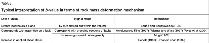
Wyss and his co-workers (Wyss et al., 1997) pointed out that mapping the b-value is equivalent to mean magnitude and assumes that this is proportional to the mean crack length. They also point out that along fault zones the low b-values seem to correspond with asperities (Amelung and King, 1997; Wiemer et al., 1998; Wiemer and Wyss, 1997), while high b-values correspond with creeping sections of faults. High b-values seem to be a characteristic of active magma chambers (Wiemer et al., 1998; Wyss et al., 1997) where seismicity is dominated by the creation of new fractures under stress build-up.
Mogi (1962) noted that increasing material heterogeneity results in a high b-value, while others have pointed out that an increase in applied shear stress (Scholz, 1968; Urbancic et al., 1992; Wyss et al., 1997) or an increase in effective stress decreases the b-value (Wyss, 1973; Wyss et al., 1997).
In the mining environment different b-values have been associated with different rock mass failure mechanisms. Legge and Spottiswoode (1987) pointed out that higher b-values may be expected to result from seismic events occurring on different planes dispersed in a three-dimensional volume, while lower b-values will be associated with events distributed uniformly in two dimensions, as on a single plane. Further along the scale, very low b-values can be associated with one-dimensional linear distributions, which could result from the interaction between the mining-induced stress change and extensive planar discontinuities.
The b-value has in some cases been linked to a fractal dimension, D. Aki (1981) related the b-value and the fractal dimension as D = 2b. The conclusions of Spottiswoode and Legge are consistent with a fractal interpretation of the b-value, where a b-value of 0.7 would relate to a D of 1.5, which could be interpreted as planar spatial distribution of events; and a b-value of 1.5 relates to a D of 3, which could be associated with a three-dimensional distribution of events.
The spatial assessment of the b-value is, therefore, valuable for both hazard assessment and the interpretation of the rock mass response to mining.
A generalized and simplified summary of the literature on the interpretation of the b-value is provided in Table I.
Evaluation of the spatial variation of b-value
In order to evaluate the spatial variation of b-value, a grid is generated over the volume of interest and the b-value obtained for every grid point. Several crustal seismology studies were performed where the spatial variation in b-value was evaluated (e.g. Wiemer et al., 1998; Wiemer and Wyss, 1997; Wyss et al., 1997). These studies used the methods developed by Wyss and co-workers that are incorporated into a Matlab library (Zmap) (Wyss et al., 1997). The methodology presented here is, in general terms, similar to the approach used by Wyss and his co-workers.
The method used in this study can be summarized as follows:
► Events with magnitudes much smaller than the estimate of the overall sensitivity based on the whole data-set (mmin - Δ) are excluded from the analysis. This is done to speed up the calculations by excluding very small events that do not contribute to obtaining the b-value. Including these very small events also has a negative impact on the overall algorithm performance as it reduces the number of events useful for b-value calculations within the search distance Rmax from each grid point
► For each grid point, the mmin and b-value are obtained from the closest N points and calculated with the search radius limited to a value Rmax. Rmax is a user-defined value which depends on the resolution of the data, the data density, and the purpose of the analysis.
With this method, only the maximum search distance is specified and the real search distance is determined by the distance to the Nth neighbouring event. Each grid point therefore has a unique search distance. This is illustrated in Figure 1, where the sizes of the spheres illustrate the search volume with radius Rmax.

A user-defined Rmax value limits the analysis to be performed on grid points with N or more values within a radius smaller or equal to Rmax, the purpose of which is to restrict the grid point b-value to local data.
Several quality checks are built into the analysis, which are discussed in the sister paper (Wesseloo et al., 2014). In addition to these, the following checks are also implemented in relation to the b-value assessment:
► The value of mmin must be within reasonable expected bounds
► The number of events with magnitude greater than mmin must exceed a set threshold value.
This added quality check is necessary to ensure that reasonably stable b-values are obtained, as the standard deviation of the b-value is inversely proportional to the square root of the number of events used in the b-value calculation (the number of events above mmin) (Kijko and Funk, 1994), i.e.:

Algorithm for finding mmin and b for a given subset of data
In order to obtain the grid-based spatial distribution of the b-value, I developed an algorithm to automatically obtain the mmin and b-value for the subset of data associated with every grid point. Examples of the results obtained by the algorithm are shown in Figure 2.

The algorithm aims to maximize the number of data points included above mmin, while minimizing the deviation from the log-linear GR relationship. This described process is performed for any data-set for which the mmin and b-value need to be obtained.
The process for obtaining mmin can be described as follows:
► Sort the data-set of magnitudes in descending order
► Calculate the b-value for subsets of the data, where each subset of data is defined as consisting of data points 1 to k where k varies between 10 and the full number of data points in the data set. The b-value for each subset, i, is therefore defined as follows:
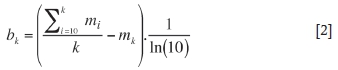
► The minimum value of k = 10 is an arbitrarily chosen practical lower limit and can be set higher. The purpose of this minimum value is simply to ignore erratic behaviour for the very high tail end of the distribution
► For each subset k, obtain the Kolmogorov-Smirnov goodness of fit parameter, KS. This parameter is not sensitive to the exponential tail end of the distribution and is, therefore, well suited for the stable estimation of mmin
► The decision parameter, C, is defined as follows:

The decision parameter has the form (A • B) • (C), with each of these components combined to provide a good and stable estimate of mmin.
A gives more weight to steeper b-values. This component mitigates against the search algorithm overshooting the true mmin value as a result of a balancing effect of residual values on both sides of the best-fit relationship near the mmin value.
B gives more weight to more data included above the mmin value and works against local minimum values for small values of k.
C defines the goodness of fit, with larger values defining a better fit
► The value of k for which Ck is a maximum defines the number of data points in the full data-set. That is:

Independent check for the algorithm
Check on the second moment
Figure 3a shows the result of the mmin algorithm applied to data from an Australian mine. The dashed lines show the GR relationship for b ± σb. The change in the decision parameter is shown in Figure 3b. Figure 3c shows the first and second moment values of the distribution with mmin assumed to be at each of the event magnitude values. This graph serves as an independent check of the algorithm.
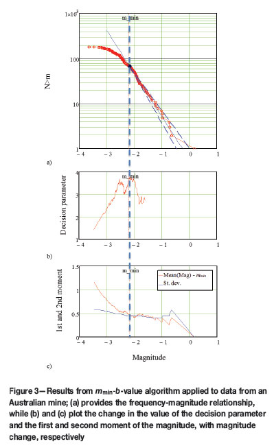
Figure 3c shows the 1st and 2nd moment values of the distribution with mmin assumed to be at each of the event magnitude values. For a negative exponential distribution, the first and second moments (mean and standard deviation of the distribution) are equal.
It should be recognized that the open-ended GR relationship is the negative exponential distribution of the translated values of (Magnitude - mmin).
For the GR relationship, therefore, the translated first and second moments should be equal. The change in the calculated first and second moments of the data-set is shown in Figure 3c. In this case, the algorithm estimate of mmin is at the smallest magnitude before the values of the first and second moments start to deviate from each other. That is the smallest value of mmin at which the distribution exhibits the characteristics of a negative exponential distribution. As the second moment is not used in the mmin algorithm, this provides independent support for the reliability of the algorithm.
Algorithm verification using synthetic data-sets
In order to verify the developed algorithm, synthetic data-sets were generated. These enable the known values of the b-value and mmin to be compared with those obtained automatically through the use of the proposed algorithm.
To generate the synthetic data-set, random deviate sampling was performed from a specified Truncated GR relationship. This data-set was randomly distributed in a rectangular volume with an arbitrary chosen array of sensors. The distance between the event and sensor location was used to determine which events will be detected by the system. The resulting data-set provides one data sample for testing the proposed algorithm.
The abovementioned process was repeated several hundred times to obtain the distributions of mmin and b-values. Two examples are shown in Figure 4.
In the figure, a histogram of the estimated mmin values is shown in blue on the chart on the right side. Also shown in the right hand chart is one of the several hundred sampled data-sets in red, together with its corresponding mmin value as a black dot on the curve and the fitted GR relationship as a solid blue line.
The distribution of mmin values follows a fairly narrow distribution around the true value.
On the left side in Figure 4, a histogram of estimated b-values is shown in green. The distributions of b-values follow a normal distribution around the specified b-value. It should be noted that a variation in the estimated b-value will result from the fact that each of the samples provides only a small portion of the true population. This can be seen in Figure 5. The solid green histogram shows the variation in the estimated b-value obtained from the data-set for which the mmin value is estimated, while the open blue histogram shows the distribution of results for which the true mminvalue is specified.
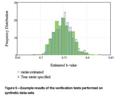
The similarity in the distributions confirms the reliability of the method for obtaining a good GR relationship for the data-set. Note that it is not implied that same b-value is always obtained for the two cases, but that the inherent uncertainty in the b-value is not increased by applying the algorithm to calculate mmin.
Results of evaluation of the spatial variation of b-value
The method described previously was applied to the database of Tasmania Mine (formerly known as Beaconsfield). Figure 6 shows the isosurfaces enveloping the higher, intermediate, and lower b-values for different dates during the history of the mine. The green volume indicates b > 1.2, orange indicates 0.8 < b < 1.2, and red b < 0.81. The volume covers changes over time as mining progresses and the seismically active volume increases.

This method clearly demonstrate that the b-value changed over time for different areas. Some areas show a high b-value which reduces as mining progresses, and later increases with further progressing of the mining. The original high b-value is associated with fracturing taking place as stress change occurs. With further mining deformation mechanism is dominated by larger structures with an associated lower b-value. At later stages in the mining, the stresses on these structures are released and the seismicity takes the form of continued fracturing in the hangingwall.
This is similar to the results reported for a deep-level South African environment by Legge and Spottiswoode (1987). In contrast to some of the other areas, the western (left) abutment continues to exhibit a low b-value throughout the mining history. This implies that seismic deformation in this area is typically concentrated on major structures.
Concluding remarks
The b-value of seismicity has been linked to the seismic deformation mechanism of the rock mass and as such is important for quantitative seismology in mines. The spatial and temporal evaluation of the b-value is important for the evaluation of the rock mass response to mining and changes in seismic hazard as a result of mining.
The evaluation of the spatial variation of the b-value was successfully implemented on a grid basis with an automated method for obtaining the mmin and b-value for subsets of data.
Acknowledgements
My sincere appreciation to Mr William Joughin and Professor Ray Durrheim for reviewing the paper. I thank the following organizations who provided funding for this research through the Mine Seismicity and Rockburst Risk Management project: Barrick Gold of Australia, BHP Billiton Nickel West, BHP Billiton Olympic Dam, Independence Gold (Lightning Nickel), LKAB, Perilya Limited (Broken Hill Mine), Vale Inc., Agnico-Eagle Canada, Gold Fields, Hecla USA, Kirkland Lake Gold, MMG Golden Grove, Newcrest Mining, Xstrata Copper (Kidd Mine), Xstrata Nickel Rim, The Minerals Research Institute of Western Australia.
References
Aki, K. 1981. A probabilistic synthesis of precursory phenomena. Earthquake Prediction, an International Review. Maurice Ewing Series, vol. 4. [ Links ] Simpson, D.W. and Richards, P.G. (eds.). American Geophysical Union, Washington. pp. 566-574. [ Links ]
Amelung, F. and King, G. 1997. Earthquake scaling laws for creeping and non-creeping faults. Geophysical Research Letters, vol. 24. pp. 507-510. [ Links ]
Kijko, A. and Funk, C. 1994. The assessment of seismic hazards in mines. Journal of the South African Institute of Mining and Metallurgy, vol. 94, no. 7. pp. 179-185. [ Links ]
Legge, N. and Spottiswoode, S. 1987. Fracturing and microseismicity ahead of a deep gold mine stope in the pre-remnant and remnant stages of mining. 6th ISRM Congress, Montreal, Canada. Balkema, Rotterdam. pp. 1071-1077. [ Links ]
Mogi, K. 1962. Magnitude-frequency relation for elastic shock accompanying fractures of various materials and some related problems in earthquakes. Bulletin of the Earthquake Research Institute, University of Tokyo, vol. 40. pp. 831-853. [ Links ]
Sammis, C., Nadeau, R., Wiemer, S., and Wyss, M. 2004. Fractal dimension and b-value on creeping and locked patches of the San Andreas Fault near Parkfield, California. Bulletin of the Seismological Society of America, vol. 94. pp. 410-421. [ Links ]
Scholz, C. 1968. The frequency-magnitude relation of microfracturing in rock and its relation to earthquakes. Bulletin of the Seismological Society of America, vol. 58. pp. 399-415. [ Links ]
Urbancic, T.I., Trifu, C.I., Long, J.M., and Young, R.P. 1992. Space-time correlations of b-values with stress release. Pure and Applied Geophysics, vol. 139. pp. 449-462. [ Links ]
Wesseloo, J. 2013. Towards real-time probabilistic hazard assessment of the current hazard state for mines. Proceedings of the 8th International Symposium on Rockbursts and Seismicity in Mines. Saint-Petersburg -Moscow, pp. 307-312. [ Links ]
Wesseloo, J., Woodward, K., and Pereira, J. 2014. Grid based analysis of seismic data. Journal of the Southern African Institute of Mining and Metallurgy, vol. 114, no. 10. pp. 815-822. [ Links ]
Wiemer, S., McNutt, S., and Wyss, M. 1998. Temporal and three-dimensional spatial analyses of the frequency-magnitude distribution near Long Valley Caldera, California. Geophysical Journal International, vol. 134. pp. 1-13. [ Links ]
Wiemer, S. and Wyss, M. 1997. Mapping the frequency-magnitude distribution in asperities: An improved technique to calculate recurrence times? Journal of Geophysical Research, vol. 102. pp. 15115-15128. [ Links ]
Wyss, M. 1973. Towards a physical understanding of the earthquake frequency distribution. Geophysical Journal of the Royal Astronomical Society, vol. 31. pp. 341-359. [ Links ]
Wyss, M., Shimazaki, K., and Wiemer, S. 1997. Mapping active magma chambers by b-values beneath the off-Ito volcano, Japan. Journal of Geophysical Research, vol. 102. pp. 20413-20422. [ Links ]
This paper was first presented at the, 6th Southern African Rock Engineering Symposium SARES 2014, 12–14 May 2014, Misty Hills Country Hotel and Conference Centre, Cradle of Humankind, Muldersdrift.
1 Note that these isosurface values were chosen for the local magnitude scale used on site, which tends to give lower b-values than for moment magnitude

