6TH SOUTHERN AFRICAN ROCK ENGINEERING SYMPOSIUM

 

Grid-based analysis of seismic data

 

 

J. Wesseloo; K. Woodward; J. Pereira

Australian Centre for Geomechanics, The University of Western Australia, Australia

 

 

---

SYNOPSIS

Quantitative seismology is an important tool for investigating mine-induced seismicity and the quantification of the seismic rock mass response. The spatio-temporal interpretation of seismic data within an ever-changing three-dimensional mining environment provides some challenges to the interpretation of the rock mass response. A grid-based approach for the interpretation of spatial variation of the rock mass response provides some benefits compared with approaches based on spatial filters. This paper discusses a grid-based interpretation of seismic data. The basic methods employed in the evaluation of the parameter values through space are discussed and examples of applications to different mine sites given.

Keywords: quantitative seismology, mine induced seismicity, rock mass response, spatial evaluation.

---

 

 

Introduction

Seismographs were first installed to monitor mining-related seismicity in South Africa in 1910. The first in-mine seismic systems were installed in the 1960s, mainly for research purposes. Intensive research, development, and commercialization during the 1990s led to the widespread implementation of real-time digital monitoring systems and quantitative methods of analysis (Durrheim, 2010; Mendecki et al., 1997).

Since then, the understanding of mine-induced seismicity and the quantification of the seismic rock mass response has formed the basis of seismological analysis and seismic hazard mitigation in South Africa. This principle of quantifying and understanding the rock mass deformation and failure mechanism has been introduced in other countries in different forms and focused on different mining environments. Potvin and Wesseloo (2013) point out that the mines in Australia, Canada, and Sweden tend to have more complex three-dimensional orebodies and are generally smaller and much more contained compared to the seismically active South African mines. For that reason it is easier to install a more sensitive three-dimensional array to cover the mine volume. With the more sensitive systems in Australia, Canada, and Sweden, local rock engineers tend to focus on the overall rock mass response to mining based on accurate source location and the analysis of populations of seismic events with magnitude of completeness as small as ML-2. A grid-based spatial analysis of seismic data was developed to improve and simplify quantitative seismological interpretation within this environment. The methods, however, have broader application.

Funk et al. (1997) presented work on the visualization of seismicity that resulted in the systems for generating contours and isosurfaces of seismic parameters. The work presented here generalizes and extends the concepts used in that work.

 

Analysis with spatial filters

Seismic events tend to cluster at the locations of active seismic sources where some form of dynamic failure process occurs. The identification and understanding of seismic sources is important in seismic risk management in that they may be, or become in the future, the cause of significant seismic hazard. In particular, small events may start to form clusters at an early stage of extraction, with a relatively small stress change. When the seismic system is sensitive enough to capture small events, this can assist in the timely identification of seismic sources and allow for the tracking of how these sources respond to mining and, more specifically, how seismic hazard related to these sources evolves as extraction progresses.

Interpretation of the character of seismic sources in space and time is generally done by analysis of some spatially sub-filtered data-set. This sub-filtering is often simply based on a three-dimensional volume in space (polygon). In Australia, Canada, and Sweden, the data is often sub-filtered on clusters.

The most widely used clustering method is probably that implemented in the software mXrap (formerly known as ms-rap) based on the Comprehensive Seismic Event Clustering (CSEC) technique described by Hudyma (2008). The CSEC method is a semi-automated two-pass approach, which was developed on the basis of generic clustering techniques: CLINK and SLINK (Jain et al., 1999, Romesburg, 2004). The first pass of clustering using CLINK is totally automated, and clusters together events based exclusively on spatial criteria. The CLINK clusters are then submitted to a second pass of processing, where clusters are selectively grouped into 'cluster groups' representing individual seismic sources. This cluster grouping is a manual process that requires interpretation of the likely seismic sources at the mine and a sound knowledge of the geology and the induced stress conditions. Cluster grouping is generally based on the similarity of source parameters, the spatial proximity of clusters, and on the correlation of the location with known geological or geometric features.

The cluster grouping process can be seen as building a seismic source model by using the generated clusters as basic building blocks. In this sense it is similar to analysing an area with the use of polygons, as the polygons become the basic units within the seismic source model. The use of a spatial filter (cluster groups or polygons) to provide a basic spatial unit for quantitative seismic analysis is a common and practical approach. This, however, introduces a bias of interpretation towards the pre-defined polygon as the polygon is originally chosen by the analyst based on preconceived ideas. This process is, per se, subjective, and the value depends to a large degree on the understanding and training of the person performing this analysis. Subjectivity, however, is part of geotechnical engineering and attempting to eliminate subjectivity from geotechnical analysis is a futile exercise. With the grid-based approach, however, we can aim to reduce interpretation bias by providing a spatial interpretation of the data that is independent of any chosen spatial filter.

Having said this, one has to recognize that the grid-based interpretation is not free of user influence as it also is influenced by the chosen analysis parameters. It is our conviction, though, that the nature of the analysis parameters, and the ease of testing the influence on the analysis parameters on the results, leads to a systematic reduction in personal bias.

 

Grid-based analysis of seismic data

In the grid-based approach, the seismic source parameters are assessed through space by interpolating the source parameters. This approach allows for anomalies to be identified without prior selection of groups or polygons. This is illustrated in Figure 1 and Figure 2.

 

 

 

 

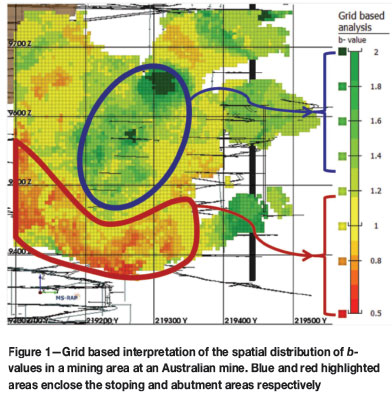
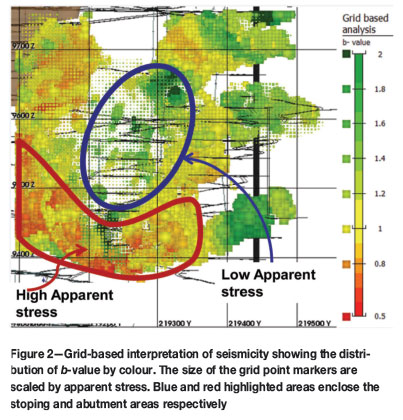
Figure 1 shows the spatial distribution of b-values at an Australian mine. High values occur around the stoping volumes while low b-values occur at the lower abutment. These differences can be related to the difference in the source mechanism in these areas; the higher b-values correspond with stress fracturing seismicity, and the lower b-values relate to a shear mechanism.

The same plot is combined with a spatial distribution of apparent stress in Figure 2. The colouring of each grid point in space is the same as that in Figure 1, but in Figure 2 each grid-point marker is scaled by the geometric mean of the apparent stress. The apparent stress is proportional to the mean shear stress at the source of the event (McGarr, 1994). The areas of the mine showing higher b-values generally show a low apparent stress, while the lower abutment area shows a high apparent stress state corresponding with low b-values. In this example, the distribution of b-values through space can be obtained without a pre-defined model of rock mass response.

 

General principle

The general principle behind the grid-based approach for quantitative mine seismology can be summarized as follows:

Assign a representative seismic parameter value to grid points in space based on the events in its neighbourhood in order to extract information from the variation of these different parameter values in space.

Added value is obtained from this approach when the different parameters are retained on each grid point, which allows for the analysis of these different parameters together as shown later.

What can be regarded as 'representative' and 'the neighbourhood' depends on the purpose of the analysis, the density and quality of the seismic data, and the type of parameter interpolation that is performed i.e. obtaining the cumulative parameter assessment, interpolation of the mean value, or obtaining the b-value.

The neighbourhood is defined by assigning a maximum influence distance, with the addition of two more quality checks. For a grid point to be assigned a representative seismic parameter, the grid point events around it must be both close enough and dense enough. This is illustrated in Figure 3. The condition that events must be dense enough in the vicinity of the grid-point prevents the transfer of parameter values from areas further away, with dense data, to a grid point where the density of the events close to the grid point does not warrant the calculation of a parameter value.

 

 

Grid-based analysis of seismic data

The grid-based interpretation of seismic data requires different approaches for different types of parameters, whether it is the mean or cumulative value of a parameter that is of interest, or the b-value.

It is important to note that in all the different approaches, the gridding process involves some level of smearing, the degree of which is dependent on the analysis parameters that are discussed in this paper. It is important that the resolution of the interpretation should match the resolution of the original input data. Sparse data-sets would require more smearing than high-resolution dense data-sets. A simple sensitivity analysis should be performed to test the sensitivity of the outcomes to chosen input parameters.

Obtaining a grid-based interpretation of b-value

The b-value of the frequency magnitude distribution is proportional to the mean of the magnitude and, as such, is simply a statistical parameter. The appropriate b-value cannot be obtained without knowledge of the magnitude of completeness of each subset of data. For this reason, the method for obtaining the spatial distribution of the b-value is quite involved and is treated separately in the sister paper published in this volume (Wesseloo, 2014).

For current purposes it will suffice to summarize the process as follows. For each grid point:

► Obtain the closest N events

► For these events obtain the m_min and associated b-value

► Retain b-values for grid points passing the quality tests.

Mean value of all parameters

In order to obtain the mean value of parameters, the geometric mean of the parameters of the closest events to each grid point is calculated. The process can be summarized as follows. For each grid point:

► Find all the events (if > N) within a distance R_min or the closest N events within a seach distance of R_max

► Calculate the geometric/arithmetic mean for the parameter

► Perform quality checks (see above) and retain calculated values for only the grid points passing the quality tests.

This approach is used for obtaining spatial distribution of parameters like energy index (EI), apparent stress (AS), and time of day (TOD).

Smearing cumulative parameters

In the cases where one is interested in the cumulative effect of different events, for example to obtain an event density or the cumulative apparent volume, a smearing process is used. In contrast to the method used to obtain the mean parameter of neighbouring events (previous section), the parameter value (intensity, I) of each event is distributed to (or 'smeared onto') grid points within its zone of influence.

This procedure can be summarized as follows:

► For each event

- Find all grid points within its influence zone

- Distribute a portion of its value to every grid point

► For every grid point

- Sum all the portions received from each event

- Perform quality checks.

This is performed with a variable smoothing where the kernel bandwidth is linked to the event source size.

The distribution of the events' parameter is performed with an inverse distance weighting. The cumulative parameter at each grid point is obtained as the sum of all the values of all the events registered to that grid point. This can be expressed as follows:

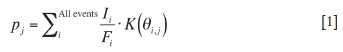
where p_j is the cumulative parameter at grid point j, and s are the location vector of the event and grid points. The intensity value, I, is the parameter value of interest and K(θ) is the kernel function. The bandwidth function h defines the influence zone of each event, i.

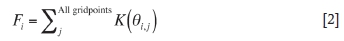
F is a correction factor that ensures that no errors are introduced due to the discretization of the volume space, i.e that the following condition is met:

In other words, summing the parameter values over all events must equal the sum of the parameter value associated with each of the grid points.

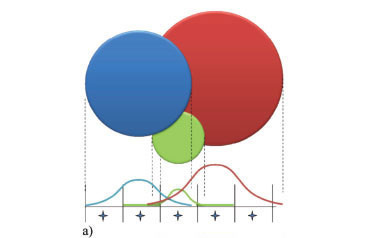
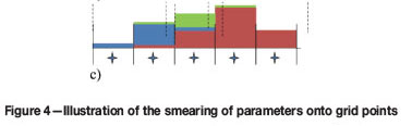
This process is graphically illustrated in Figure 4. The circles in Figure 4a represent different events with different source sizes. The parameter values of each of these curves are distributed to the grid points in the influence zone with the kernel function (Figure 4b). These values for each grid point sum to the final spatial distribution of the parameter value (Figure 4c).

 

 

In the smearing process, described in the following section, each event has an influence zone. Our current approach is to define an influence based on the event source radius, as defined by Brune (1970). A lower cut-off value equal to the grid spacing is imposed to ensure stability of the method for coarser grid discretization. A limiting ceiling value is also introduced for numerical efficiency and stability. The results are not sensitive to the ceiling value.

It is important to note that the results of the smearing process are not sensitive to the influence of large events, as the parameter values of these large events are distributed to more grid points within the larger influence zone.

 

Grid-based quantitative analysis

This section provides a short discussion on some of the parameters used in the grid-based analysis and examples to illustrate the application of the method. The use of these methods is not limited to these parameters.

Energy stress and apparent stress

Apparent stress is generally calculated as:

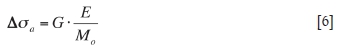
where G is the shear stiffness of the rock mass, and E and M_o are the total radiated energy and average moment for an event, respectively. As indicated by its name, the definition of apparent stress relates to the stress state in the rock mass at the occurrence of the event. The apparent stress is proportional to the mean shear stress at the source of the event, (McGarr, 1994), and is defined as follows:

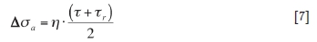
where η is the seismic efficiency and τ and τ_r are the peak and residual shear stress, respectively.

As η is unknown, the absolute shear stress is also unknown. The value of apparent stress is, however, a good indicator of the relative stress state. This concept is refined by Mendecki (1993), who showed that for a given slope of the log(E)-log(M) relation, the intercept value relates to the stress level. A simpler way to express this relative value of the intercept is the log(EI), as defined by van Aswegen and Butler (1993).

Obtaining the log(E)-log(M) trendline introduces some difficulties with unsatisfactory 'best-fit' lines. This problem can easily be overcome. For the sake of maintaining the focus of this paper, this will be discussed further in Appendix A.

The results of a grid-based analysis of the log(EI) at an Australian mine are shown in Figure 5. The colour scale of the grid points reflects the values of log(EI). The transparency of the grid points is also scaled with log(EI). The upper 50% of the log(EI) values are more solid while the lower 50% are more transparent.

 

 

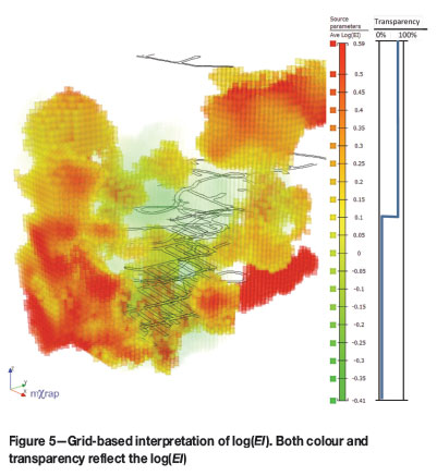
In this particular case, low log(EI) values occur at the centre of the volume with surrounding higher log(EI) values. This corresponds with lower stress areas in the immediate vicinity of the mined stopes, while the more competent rock further away from the stopes is under a higher stress state. The particular shape of the grid cloud is determined by the location of seismic data, as grid points are generated only where seismic data exists.

Time of day

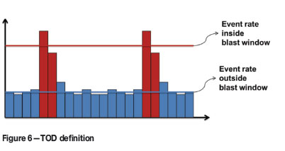
The time-of-day parameter (TOD) is a measure of the temporal differences in the seismic response. It is defined as the ratio of the rate of seismicity occurring within a specified time window(s) to the rate of seismicity occurring outside of those time windows. As an example, where the rock mass reacts strongly (in a purely temporal sense) to blasts, the TOD value will be high for a time window around blast time. Orepass noise, on the other hand, results in TOD values of less than 1 for time windows around shift change, as no orepass activity occurs during shift change.

 

 

Grid points with a low TOD were isolated for an Australian mine. These grid points all located in a couple of distinct areas. The diurnal chart for the events reporting to these grid points is shown in Figure 7. From this chart it is clear that the events are small and inversely correlated to the shift change, indicating that these events are human-induced noise, in this case orepass noise. The fact that these events are human-induced noise is highlighted by the fact that the time of lunch breaks during the two shifts is visible in the diurnal chart.

 

 

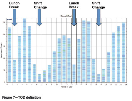
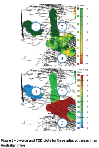
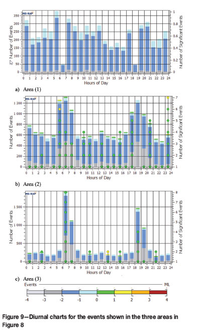
Figure 8 shows the b-value and TOD plots for three adjacent areas in a mine. Area (1) has an unnaturally high b-value with a very low TOD and is the result of crusher noise. Area (2) has a very high b-value and a higher TOD and is the result of a raise bore experiencing some dogearing. Area (3) has a lower, but still fairly high, b-value, with a very high TOD. The seismicity in this area generally relates to stress fracturing around development blasting temporally concentrated around blast time. The diurnal charts for these three areas area shown in Figure 9.

 

 

 

 

Cumulative damage

It is generally accepted that there is a correlation between historical seismic activity in an area and the damage accumulated in the rock mass. Despite the work of Falmagne (2001), Cai et al. (2001), Coulson and Bawden (2008), and Pfitzner et al. (2010), there appears to be no accepted way to quantify this damage accumulation from seismic data. Until these difficulties are solved, we propose the use of apparent volume and the cube root of moment as proxies for damage.

Apparent volume has been linked to the amount of coseismic strain (Mendecki, 1997), while the cube root of moment is proportional to the maximum displacement at the seismic source (McGarr and Fletcher, 2003).

Figure 10 shows the results of a grid-based analysis at an Australian mine. In this example, log(EI) as a proxy for stress and the cube root of moment as a proxy for damage are combined. Log(EI) is represented by the colour scale and the transparency varies with damage. The mean log(EI) is calculated for a 6-month data period, while the damage is accumulated over the whole history of the mine.

 

 

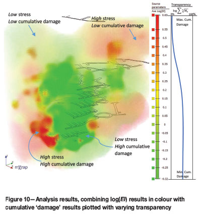
The destressed area in this case corresponds with the area of high historical damage, with some high-stress areas on the abutments, where similar levels of damage have accumulated. It should be noted that the destressing did not take place due to the damage alone but is a result of the mining voids. As one would expect, the area of high damage is concentrated close to the stopes.

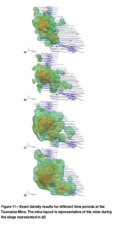
Event density

Event density is conceptually a very simple parameter and is very easy to interpret as the number of events occurring per unit volume. From a mathematical viewpoint, event density is a cumulative parameter with the intensity value, I, equal to 1 (refer to Equation [5]) and for this reason is calculated with the same method as is used for the cumulative damage.

Figure 11 shows examples from the Tasmania Mine for different time periods during the life of the mine.

 

 

Calibrating numerical models

In mining geomechanics, the need for calibrating or constraining the models with physical observations is well recognized. Seismic data provides a valuable source of information on the rock mass response to mining, and for this reason has been used by some investigators to provide calibration data for their models.

Often the calibration of numerical models with seismic data is limited to a visual correlation between the event location and strain or stress contours from the models, or the visual correlation of event density with areas of higher plastic strain. More recently, correlations between the energy release monitored within a specified cell and the modelled plastic strain energy have been used (Levkovitch et al., 2013; Arndt et al., 2013). Both of these groups limit themselves to energy and perform basic grid calculations, simply summing the energy of all monitored events located within a specific grid cell.

We are of the conviction that the grid-based approach to the evaluation of seismic data presented here provides the opportunity to better utilize the seismic data to constrain numerical models.

As the grid-based interpretation can be continually updated, this provides further opportunity to continually test predicted rock mass behaviour against experienced behaviour, with the possibility of flagging deviation from the predicted behaviour.

 

Concluding remarks

A grid-based interpretation of seismic data has been discussed and some examples of results obtained with the method presented. A grid-based interpretation allows the spatial variation of seismic source parameters to be evaluated without predetermined analysis volumes. As such, it provides some buffer against biasing of interpretations towards preconceived ideas.

The gridding process involves some level of smearing, the degree of which is dependent on the analysis parameters discussed. It is important that the resolution of the interpretation should match the resolution of the original input data. A sparse data-set would require more smearing than high-resolution dense data-sets. A simple sensitivity analysis should be performed to test the sensitivity of the outcomes to chosen input parameters.

The grid-based analysis approach is well suited to compare with results from numerical modelling approaches.

 

Acknowledgements

Our sincere appreciation to William Joughin and Professor Ray Durrheim for reviewing the paper. The following organizations provided funding for this research through the Mine Seismicity and Rockburst Risk Management project: Barrick Gold of Australia, BHP Billiton Nickel West, BHP Billiton Olympic Dam, Independence Gold (Lightning Nickel), LKAB, Perilya Limited (Broken Hill Mine), Vale Inc., Agnico-Eagle Canada, Gold Fields, Hecla USA, Kirkland Lake Gold, MMG Golden Grove, Newcrest Mining, Xstrata Copper (Kidd Mine), Xstrata Nickel Rim, and The Minerals Research Institute of Western Australia.

 

References

Arndt, S., Louchnikov, V., Weller, S., and O'hare, A. 2013. Forcasting mining induced seismicity from modelled energy release in high stress stope extraction. 8th International Symposium on Rockbursts and Seismicity in Mines, St. Petersburg and Moscow, Russia, 1-7 September 2013. pp. 267-272.         [ Links ]

Brune, J. 1970. Tectonic stress and the spectra of seismic shear waves from earthquakes. Journal of Geophysical Research, vol. 75. pp. 4997-5009.         [ Links ]

Cai, M., Kaiser, P., and Martin, C.D. 2001. Quantification of rock mass damage in underground excavations from microseismic event monitoring. International Journal of Rock Mechanics and Mining Sciences, vol. 38. pp. 1135-1145.         [ Links ]

Coulson, A. and Bawden, W. 2008. Observation of the spatial and temporal changes of microseismic source parameters and locations, used to identify the state of the rock mass in relation to the peak and post-peak strength conditions. 42nd US Rock Mechanics Symposium, San Francisco, CA, 29 June - 2 July 2008. American Rock Mechanics Association, Alexandria, VA.         [ Links ]

Durrheim, R.J. 2010, Mitigating the rockburst risk in the deep hard rock South African mines: 100 years of research. Extracting the Science: a Century of Mining Research. Brune, J. (ed.). Society for Mining, Metallurgy, and Exploration, Inc. pp. 156-171. ISBN 978-0-87335-322-9,         [ Links ]

Funk, C.W., Van Aswegen, G., and Brown, B. 1997. Visualisation of seismicity. Proceedings of the 4th International Symposium on Rockbursts and Seismicity in Mines, Kraków, Poland, 1-14 August 1997. Gibowicz, S.J. and Lasocki, S. (eds). CRC Press, Boca Raton, FL.         [ Links ]

Falmagne, V. 2001. Quantification of rock mass degradation using microseismic monitoring and applications for mine design. PhD thesis, Queen's University, Ontario.         [ Links ]

Hudyma, M. 2008. Analysis and interpretation of clusters of seismic events in mines. PhD thesis, University of Western Australia, Perth.         [ Links ]

Jain, A.K., Murty, M.N., and Flynn, P.J. 1999. Data clustering: a review. ACM Computing Surveys (CSUR), vol. 31. pp. 264-323.         [ Links ]

Levkovitch, V., Beck, D., and Reusch, F. 2013. Numerical simulation of the released energy in strain-softening rock materials and its application in estimating seismic hazards in mines. 8th International Symposium on Rockbursts and Seismicity in Mines, St. Petersburg and Moscow, Russia, 1-7 September 2013. pp. 259-266.         [ Links ]

Mcgarr, A. 1994. Some comparisons between mining-induced and laboratory earthquakes. Pure and Applied Geophysics, vol. 142. pp. 467-489.         [ Links ]

Mcgarr, A. and Fletcher, J. 2003. Maximum slip in earthquake fault zones, apparent stress, and stick-slip friction. Bulletin of the Seismological Society of America, vol. 93. pp. 2355-2362.         [ Links ]

Mendecki, A. 1993. Real time quantitative seismology in mines. Keynote Address: 3rd International Symposium on Rockbursts and Seismicity in Mines, Kingston, Ontario, 16-18 August 1993. Young, R. Paul (ed.). Barnes & Noble. pp. 287-295.         [ Links ]

Mendecki, A. 2013. Characteristics of seismic hazard in mines. Keynote Lecture: 8th International Symposium on Rockbursts and Seismicity in Mines, St. Petersburg and Moscow, Russia, 1-7 September 2013. pp. 275-292.         [ Links ]

Mendecki, A.J. 1997. Seismic Monitoring in Mines. Chapman & Hall, London; New York.         [ Links ]

Pfitzner, M., Westman, E., Morgan, M., Finn, D., and Beck, D. 2010. Estimation of rock mass changes induced by hydraulic fracturing and cave mining by double difference passive tomography. 2nd International Symposium on Block and Sublevel Caving, Perth, Australia. Potvin, Y. (ed.). Australian Centre for Geomechanics, Perth, WA.         [ Links ]

Potvin, Y. and Wesseloo, J. 2013. Improving seismic risk management in hardrock mines. 8th International Symposium on Rockbursts and Seismicity in Mines, St. Petersburg and Moscow, Russia, 1-7 September 2013. pp. 371-386.         [ Links ]

Romesburg, H.C. 2004. Cluster Analysis for Researchers. Lifetime Learning Publications, Belmont, CA. 334 pp.         [ Links ]

Van Aswegen, G. and Butler, A.G. 1993. Application of quantitative seismology in SA gold mines. 3rd International Symposium on Rockbursts and Seismicity in Mines, Kingston, Ontario, 16-18 August 1993. Young, R.P.(ed.). Balkema, Rotterdam. pp. 261-266.         [ Links ]

Wesseloo, J. And Potvin, Y. 2012. Advancing the Strategic Use of Seismic Data in Mines. Minerals and Energy Research Institute of Western Australia, East Perth, WA.         [ Links ]

Wesseloo, J. 2014. Evaluation of the spatial variation of b-value. Journal of the Southern African Institute of Mining and Metallurgy, vol. 114, no. 10. pp.823-828.         [ Links ]

 

 

This paper was first presented at the, 6th Southern African Rock Engineering Symposium SARES 2014, 12–14 May 2014, Misty Hills Country Hotel and Conference Centre, Cradle of Humankind, Muldersdrift.

 

 

Appendix A

Obtaining the log(E)-log(M) trendline

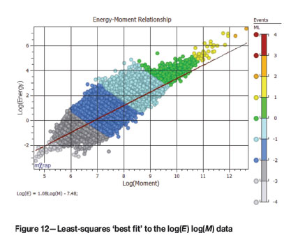
It should be recognized that a least-squares 'best-fit' approach assumes the total radiated energy (E) to be a variable dependent on the total moment (M). This assumption is incorrect as M and E are two independent parameters and as such the use of the least-squares best-fit method is invalid.

Applying the general least-squares best-fit approach to the Log(E)-Log(M) relation underestimates the slope of the trendline and overestimates the intercept (Figure 12).

 

 

When evaluating the log(E)-log(M) relationship we are not interested in obtaining log(E) as a function of log(M) but in the general statistical relationship between these parameters.

Wesseloo and Potvin (2012) suggested the use of the log(E)-log(M) quantile-quantile (QQ) relationship for this purpose, which is the method implemented in the software mXrap (Figure 13).

 

 

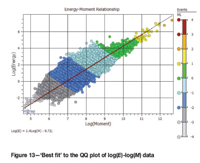
It should be noted that this approach, although much simpler, is equivalent to the approach suggested by Mendecki (2013).

The QQ method for obtaining the log(E)-log(M) relationship is performed as follows.

► Independently sort E and M, both in ascending order

► Plot log(E_i) against log(M_i) for every value of i. Note that the actual values of log(E_i) and log(M_i) are not from the same event and the only link between them is the fact that they both represent the quantile of the two different sets log(E) and log(M)

► For practical use a best-fit line can be fitted to the QQ relationship.