Factorial kriging for multiscale modelling

 

 

Y.Z. Ma^I; J.-J. Royer^II; H. Wang^III; Y. Wang^I; T. Zhang^IV

^ISchlumberger, Denver, USA
^IIUniversity of Lorraine, Nancy, France
^IIIChina University of Geoscience, Beijing, China
^IVSchlumberger-Doll Research, Cambridge, USA

 

 

---

SYNOPSIS

This paper presents a matrix formulation of factorial kriging, and its relationships with simple and ordinary kriging. Similar to other kriging methods, factorial kriging can be applied to both stationary and intrinsic stochastic processes, and is often used as a local operator. Therefore, the concepts of intrinsic random function and local stationarity are first briefly reviewed. Kriging is presented in a block matrix form in which the kriging solution is useful not only for understanding the relationships between simple and ordinary kriging methods, but also the relationships between interpolative kriging and factorial kriging. When used as a signal/noise-filtering method, factorial kriging is especially useful for multiscale modelling. Examples for general signal analysis and geophysical data signal filtering are given to illustrate the method.

Keywords: kriging in matrix form, locally stationary, block matrix, multiscale modeling, relationship between simple and ordinary kriging, filtering.

---

 

 

Heterogeneity, stationarity, and kriging

Heterogeneity is an important concern when applying a statistical method to a spatial process, because it largely determines the choice of an appropriate modelling method and whether the chosen method can be effectively applied. Large heterogeneities generally cause stationary stochastic modelling methods to go astray (Delfiner, 1976; Ma et al., 2008). Universal kriging and intrinsic random function (IRF) techniques were proposed to deal with modelling nonstationary stochastic processes (Matheron, 1973). These techniques have been successfully used for topographic mapping and other applications (Delfiner et al., 1978; Chiles and Delfiner, 2012).

Stationary, locally stationary, and intrinsic random functions

IRF theory is a generalization of stochastic processes with independent increments. The latter implies uncorrelated first-order differences, such as a Brownian motion (Matheron, 1973; Papoulis 1965; Serra, 1984). A Brownian motion is not stationary, because the variance increases when the domain of study increases. This was coined an intrinsic randomfUnction of order 0 (IRF-0) by Matheron (1973). Besag and Mondal (2005) provided a bridge between spatial intrinsic processes (also called de Wijis process) and first-order intrinsic autoregressions. By a further extension, a stochastic process whose (k+1)th differences constitute a stationary process is termed an intrinsic randomfUnction of order k or IRF-k (Matheron, 1973).

Let A denote the vector space of real measures in Rⁿ with finite supports. A second-order random function (RF) Z: Rⁿ->L²(Ù, A, P) admits a linear extension Z: A->L²(Ù, A, P) defined by

which implies the strict positive definiteness of the covariance matrix <Z(x₁), Z(x₂)> for any finite set of distinct points x1 and x₂ in Rⁿ. As an example, Wiener's linear estimator is such a type (Wiener, 1949). An IRF-k is defined in a more restrictive way. A continuous function p(x) is chosen in a way that a subspace G is defined on the space A by

As such, the linear mapping Z: G->L²(Ù, A, P) is a generalized RF on the space G.

For a nonstationary process, the covariance calculated from sample data can cause a serious bias in the prediction (Serra, 1984). Matheron defined a generalized covariance for IRF-k using the distribution theory (Matheron, 1973). It is generally difficult to characterize and construct an effective generalized covariance function in practice (Chauvet, 1989), but in most applications, the variance of the first order, called the variogram, suffices.

Stationarity of a stochastic process in a strict sense implies translation invariant of the probability density function in space or time (Papoulis 1965, p. 300). A wide sense or weak stationarity of a stochastic process assumes a constant expected value or mean and translation invariant of correlation function or variogram in space or time (Papoulis, 1965; Matheron, 1989). When applying kriging or factorial kriging with a local moving neighborhood, global stationarity is not required, but a local stationarity suffices. Local stationarity is a weaker assumption by definition (Matheron 1989, p. 126; Ma et al., 2008). Although factorial kriging can be used globally, we generally recommend using a local operator. An example is presented in a later section.

Matrix formulation of kriging

Several kriging methods have been proposed according to stationarity or non-stationarity assumptions, including simple kriging, ordinary kriging, universal kriging, and intrinsic kriging (Chiles and Delfiner, 2012). The applicability of each method depends on the physical problem of concern, and the availability of data.

Consider a random variable, Z(x), defined in a spatial domain such as:

where x is the sampling location of the variable Z(x) within the defined domain D, which is a bounded subset of the n-dimensional real space, Rⁿ.

Simple kriging

Simple kriging uses an affine linear equation for spatial prediction, such as

Because of the assumption of constant mean that can be estimated from the data, the kriging system can be obtained by minimizing the sum of the squared errors (the least-square method), and it can be expressed in the following matrix form:

where C(.) represents the covariance; CZZ is the n × n matrix of the spatial covariance of the data used for prediction, Z(x_i) to Z(x_n); cZ is the n × 1 vector of the spatial covariance between Z(x) and the data Z(xj) used for prediction; and Ask is the vector for the simple kriging weights. In an expanded form, Equation [4a] is written as

The variance, σ²_sk, of the error, ε = Z(x) - Z*(x), between the estimation and the truth can be expressed as follows:

with C_ZZ^-1 the inverse matrix of the covariance matrix C_ZZ, and the variance of Z(x).

Simple kriging is applicable to phenomena with a strong assumption of global stationarity, which implies that the global mean can be calculated from the samples. Simple kriging is especially useful for spatial stochastic simulation.

Ordinary kriging

For an IRF-0, or locally stationary random fields, the mean is not known or cannot be estimated globally by averaging the sample values. The affine Equation [3] cannot be used for estimation; an ordinary linear combination is used instead:

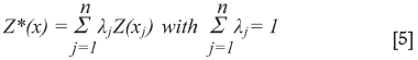
where the constraint on the kriging weights Σ_j λ_j= 1 is imposed to the estimator Z*(x) (i.e. the estimation errors being null on average, E(ε) = 0, with ε = Z(x) -Z*(x)).

The ordinary kriging system can be obtained by minimizing the sum of the square errors under the constraint in Equation [5] by using the least-square and Lagrange methods, and can be expressed in the following block matrix equation:

The error variance, σ²_ok, is equal to:

where Czz represents the sample covariance matrix, Λ_oκ is the vector of the ordinary kriging weights, u is a unit vector with all the entries equal to 1, such as u = [1 1 ... 1]^t, superscript t is the vector transpose, uok is the Lagrange multiplier due to the constraint on the kriging weights which sum to 1, and cz is the vector of covariance between the estimation point, x, and each of the sample points, xj.

Relationship between simple kriging and ordinary kriging

Equation [6a] is an expanded matrix formulation from simple kriging (see Equation [4]), taking into account the constraint on the ordinary kriging weights. The block-matrix inversion formula (Appendix 1) is used to rewrite the square matrix on the left side of Equation [6a]. The solution is thus as follows:

where Λ_sk is the vector of simple kriging weights defined in Equation [4], Λ_m is the vector of kriging weights for estimation of the mean, and ì_m the corresponding Lagrange multiplier. The latter is obtained by replacing the vector c_z with a zero vector of the same size in Equation [6a], because of the nil correlation between a random variable and its mean. λ_m is the weight of the mean in simple kriging, because Equation [3] can be expressed as

Equations [7a-d] can also be used to deduce an additive relationship among the error variances of the ordinary kriging, the local mean, and simple kriging. As the error variance σ ²m in estimating the mean is equal to -ìm (Ma and Myers, 1994), the ordinary kriging variance σ²_ok (Equation [6b]) can be expressed as a function of the simple kriging error variance and the estimation variance of the local mean:

Equations [7a-d] describe the relationship between the simple kriging weights and ordinary kriging weights, and Equation [8b] the relationship between the corresponding error variances. The ordinary kriging weights are expressed as the sum of the simple kriging weights and the ordinary kriging weights for the local mean multiplied by the weight for the mean in simple kriging. One obvious advantage of this formulation is the explicit expression of the impact of the constraint on the kriging weights. The error variance increases when using ordinary kriging because it is necessary to estimate both the local mean and the residuals.

Another advantage of Equations [7a-d] is the use of the weighting vector for the mean. By using a local operator under the local stationarity assumption, the local mean is not assumed to be known, and the estimator given by Equation [5] is equivalent to (see e.g., Matheron, 1971):

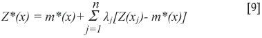
with

The kriging solution for the local mean is given in Equation [7b]. Furthermore, the estimation for the random function, Z(x), can be done with simple kriging using Equation [9], which yields the same solution as in Equations [7a-d]. In other words, the estimation of the random function by ordinary kriging is identical to the combination of the estimation of the mean using ordinary kriging and the estimation of the residual by simple kriging. This is termed the additivity theorem, which is also valid for universal kriging (Matheron, 1971; Ma, 1987). In practice, as a result of using a sliding window, m*(x) describes a low-frequency, large-scale component of the multiscale RF Z(x), which is related to factorial kriging.

 

Factorial kriging for multiple-scale modeling

Although kriging has been used most commonly for spatial interpolation, it can also be used for filtering. Typically, filtering is a decomposition based on the multiple scales of variations in a physical process. The filtering method in geostatistics is termed factorial kriging (Matheron, 1982; Ma and Royer, 1988). This method has been used in a variety of scientific applications, including signal and image processing (Ma and Royer, 1988; Wen and Sinding-Larsen, 1997; Van Meirvenne and Goovaerts, 2002), petroleum exploration (Jaquet, 1989; Du et al., 2011), soil description (Goovaerts and Webster, 1994; Bocchi et al., 2000), geochemistry (Reis et al., 2004), water resource monitoring (Yeh et al., 2006), seismic data analysis (Yao et al., 1999; Abreu et al., 2005), ecology (Lin et al., 2008), crime risk pattern analysis (Kerry et al., 2010), and health risk analysis (Goovaerts et al., 2005, 2009; Dubois et al., 2007). It assumes that the observed physical process can be interpreted as a linear combination of several sub-processes that generally exhibit different scales with different spatial dependencies, such as

where Z(x) is the RF representing the observed (though often only partially observed) physical process, Y_i(x) represents a component RF or a sub-process at a certain scale of variation, at are normalization coefficients, and T(x) is a trend function which can be approximated using orthogonal or trigonometric polynomials (Royer, 2008). The number of components q can be chosen according to the number of nested terms used in this decomposition.

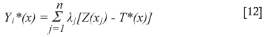
As such, factorial kriging can decompose the random process, Z(x), into several sub-processes of different scales linked with the spatial correlation structures. In theory, all the RFs, Z(x) and Y_i(x), can be an IRF-k (Matheron, 1982; Ma, 1987). Kriging prediction of these RFs can then use a generalized covariance, defined as conditionally positive definite. The predictor of the component RFs Y(x), is formed as a linear combination of known data of the original (composite) RF, such as

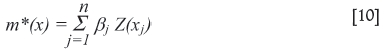
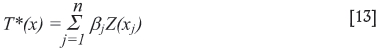
The trend function is estimated by the following linear combination:

The kriging systems used to estimate the components and the trend can be obtained by minimizing the sum of the squared errors under the constraint using the least-square and Lagrange methods, and they can be expressed in the following block matrix equations (Ma, 1987, 1993):

 

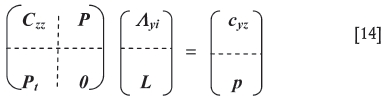
where C(.) represents the generalized covariance; Czz is the nxn matrix of the spatial covariance of the data used for prediction; Cyz is the n×l vector of the spatial covariance between Yi(x) and the data Z(xi) to Z(x_n); P and p are, respectively, the nxk matrix and k+1 vector of a chosen analytical function p(x) for fitting the nonstationary component; Λ_yi is the vector for the kriging weights; and L is a vector of Lagrange multipliers. The zero vector on the right-hand side of Equation [15] is a result of the non-randomness of the trend, T(x).

Equations [14] and [15] are the kriging systems for estimating the zero-mean component Y_i(x) and the trend T(x), respectively. Similar to the ordinary kriging system discussed earlier, the weighting vector can be obtained by using the block matrix inversion method (Appendix 1), and the solutions are

The estimation variances of the components, Y_i, and the trend, T, are given by:

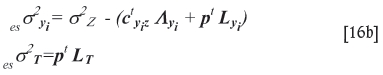
For interpolation of the original RF, Z(x), the counterpart to Equation [16a] is expressed as

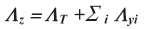
As the components, Y(x), are assumed to be orthogonal in factorial kriging, the additive relationship of covariances is such that c_z = Σc_yiz (Ma and Myers, 1994). Thus, Equations (16a) and (16b) verify the coherence condition in factorial universal kriging and factorial kriging for IRF-k:

These equations are valid for ordinary kriging but with a simplified formulation (Ma, 1993). For most applications, these components can be considered to be locally stationary. The local stationarity eases the ergodicity hypothesis, and makes the spatial prediction suitable to a local operation (Matheron, 1989).

Moreover, assuming local stationarity, all the decomposed sub-processes are estimated from the observed composite process, such as:

or in matrix form:

Where m_yi*(x) is the locally varying mean for the component Y_i(x), Z is the data vector, m_z is the locally varying mean of Z(x), and u is a unit vector with all the entries equal to 1. Because the mean is estimated, Equation [17] is not a true affine linear combination, despite its affine-like form.

 

Discussion

It is noteworthy that kriging is an exact interpolator, meaning that the kriging estimator is equal to the known value if the latter is estimated, or the sample data are all honoured (Armstrong, 1998, pp. 97-98). This is not the case for linear regression. Because factorial kriging is a probabilistic decomposition, not an interpolation by design, it is purely a filtering process at the known locations; but in the unknown locations it is also an interpolation, inherited from kriging (Ma, 1993).

The estimation of the components by factorial kriging can be considered as an ecological inference (Robinson, 1950; Wakefield, 2004), since the component processes are estimated using data from the composite or total process. It is well known that ecological inference can cause a bias in estimation (Gotway and Young, 2002; Ma, 2009). However, it is possible to objectively identify sub-processes based on the specific application by using the contextual information. For example, in image processing it is commonly useful to filter the noise and enhance the signal. The noise and signal represent different scales of variations, or different frequency contents from a viewpoint of spectral theory. Spatial filtering by factorial kriging is generally based on a nested covariance model. Some researchers have questioned the tenability of nested models (Stein, 1999, pp. 13-14). A nested covariance model may not gain much for the purpose of spatial interpolation, because of the inherent uncertainty in empirical spatial covariance or variogram for most applications. However, this is an important step for random field decomposition and signal filtering. It is tenable when combined with the contextual information, especially if the sample data are large enough. Two examples are discussed in the next section.

 

Application to signal analysis and noise filtering

In image processing, decomposition by factorial kriging is sometimes used for visual interpretation, either for filtering noise or extracting a specific feature (Ma and Royer, 1988; Wen and Sinding-Larsen, 1997). Here, an example of filtering noise and extracting signal illustrates how to simultaneously model two differently-scaled spatial heterogeneities. The factorial kriging works for any number of components for different scales as shown in Equation [11], but the examples presented here include two components only.

Kriging with an unknown mean, either stationary or nonstationary, for a two-component model can be represented by a signal plus an additive noise model:

where S(x) represents a larger-scale-component random function, N(x) represents a smaller-scale-component random function, and Z(x) represents the composite random process.

Modelling the three random functions can be performed simultaneously using the sampling data of Z(x).

Note that as a result of non-bias constraint on the estimators, the sum of the weights for all sample points and the mean is equal to unity, whereas the sum of the weights for the noise is equal to zero. The weighting function can be considered as a transfer function.

Figure 1 shows an example of filtering the noise in image processing. The Lena picture is widely used in 2D signal analysis for noise filtering and feature detection. First, the variogram of the noisy digital picture (Figure 1a) was calculated, and then the calculated variogram was fitted into a theoretical model (Figure 1b), including a nugget effect of 365 intensity in square (IIS), an exponential variogram with the sill equal to 570 IIS and the range equal to 10 pixels, an exponential variogram with the sill equal to 1270 IIS and the range equal to 27 pixels, and a spherical variogram with the sill equal to 620 IIS and the range equal to 36 pixels. The nugget effect component in the variogram at the origin is due to the presence of white noise. Factorial kriging is used to filter out the noise by eliminating the nugget effect. Specifically, using the matrix notation under the local stationary model (Equation [18]), the signal weighting vector is simply a combination of the two forms in Equation [16], but with simplification to a locally stationary model, such as

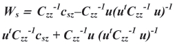
where C_ZZ represents the spatial covariance matrix for the noisy picture, and csz is the vector of spatial covariance between the noisy picture and the signal. All other terms are defined in Equations [7a-d]. The spatial covariance or correlation terms are calculated from the variogram in Figure 2b using the following relations (Journel and Huijbregts, 1978):

where C(h) is the covariance, C(0)) = ó2 the variance, and ã(h) the variogram of the spatial variable Z(x).

Figure 1c shows the denoised picture (i.e., the signal component of the noisy picture in Figure 1a). In this application, the noise is not of interest, and thus is not shown. The signal contains several different scales of information related to not only the two exponential variograms and one spherical variogram stated above, but also the locally varying mean or the trend that is expressed by Equation [10] or [13]. In other words, the signal itself still has several scales of information.

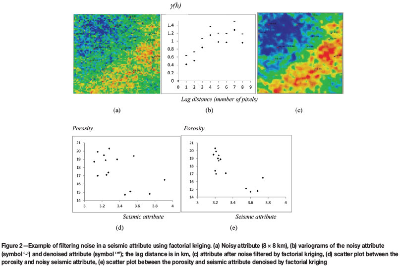
Another example of filtering noise, in a seismic attribute, is shown in Figure 2. The noisy attribute had a correlation coefficient of 0.53 with the measured porosity. After filtering out the noise using factorial kriging by eliminating the nugget-effect component, the correlation was improved to 0.79. This is because the noise component had no correlation to the porosity as the noise represents the smallest-scaled component, and removing it is equivalent to matching the more correlated parts of the two variables. In this sense, factorial kriging is a disaggregation that enables the identification of the scale of information and thus provides a means for matching the scale between the two variables.

 

Concluding remarks

Kriging was initially developed as an interpolation method dealing with stationary or mild non-stationary (IRF-0) processes. With many extensions, there are now a variety of kriging methods to deal with multiscale problems of natural phenomena, including universal kriging, IRF-k, and factorial kriging. Although IRF-k is theoretically elegant, it is often difficult to use, and does not always give good results, often because of an inadequate identification of the complexity of heterogeneities (Ma, 2010). Defining a multilevel model based on the hierarchy of scales can deal with multiscale problems more effectively for many applications (Ma et al., 2009). In such a framework, factorial kriging offers a filtering technique that explicitly decomposes the composite phenomenon of multiple scales into component processes. In some cases, even ordinary kriging, if a local neighborhood is utilized, can be used to deal with two-scale problems as shown by Equation [7]. These methods are also applicable to multivariate geostatistics that involves multiple physical variables (Wackernagel, 2003).

 

Acknowledgements

The authors thank Schlumberger Ltd for permission to publish this work, and Dr David Psaila for reviewing an early version of the draft. Dr. Hongliang Wang is the correspondence author, and his work was partly funded by the National Natural Science Foundation (Grant No. 91114203) and the National Science and Technology Major Projects framework.

 

References

Abreu, C.E., Lucet, N., Nivlet, Ph., and Royer, J.J. 2005. Improving 4D seismic data interpretation using geostatistical filtering. Reservoir Monitoring and Management, 9 th International Congress of the Brazilian Geophysical Society. SBGf, Bahia. pp. 289-294.         [ Links ]

Armstrong, M. 1998. Basic Linear Geostatistics. Springer, Berlin. 166 pp.         [ Links ]

Besag, J. and Mondal, D. 2005. First-order intrinsic autoregressions and the de Wijs process. Biometrika, vol. 92, no. 4. pp. 909-920.         [ Links ]

Bocchi, S., Castrignano, Á., Fornaro, F., and Maggiore T. 2000. Application of factorial kriging for mapping soil variation at field scale. European Journal of Agronomy, vol. 13. pp. 295-308.         [ Links ]

Bourgault, G. 1994. Robustness of noise filtering by kriging analysis. Mathematical Geology, vol. 26, no. 6. pp. 723-734.         [ Links ]

Chauvet, P. 1989. Quelques aspects de l'analyse structural des FAI-k a 1-dimension. Geostatistics. Armstrong, M. (ed.). Kluwer, Dordrecht. pp. 139-150.         [ Links ]

Chiles, J.P. and Delfiner, P. 2012, Geostatistics: Modeling Spatial Uncertainty. John Wiley & Sons, New York. 699 pp.         [ Links ]

Delfiner, P. 1976. Linear estimation of nonstationary spatial phenomena. Advanced Geostatistics in the Mining Industry. Guarascio, M., David, M., and Huijbregts, C. (eds.). Riedel, Dordrecht. pp. 49-68.         [ Links ]

Delfiner, P., Renard, D., and Chiles J.P. 1978. BLUEPACK-3D Manual. Centre de Geostatistique. Ecole des Mines, Fontainebleau, France.         [ Links ]

Du, C., Zhang, X., Ma, Y.Z., Kaufman, P., Melton, B., and Gowelly, S. 2011. An integrated modeling workflow for shale gas reservoirs. Uncertainty Analysis and Reservoir Modeling. Ma, Y.Z. and La Pointe, P. (eds.), American Association of Petroleum Geologists, Memoir 96.         [ Links ]

Dubois, G., Pebesma, E.J., and Bossew, P. 2007. Automatic mapping in emergency: a geostatistical perspective. International Journal of Emergency Management, vol. 4, no. 3. pp. 455-467.         [ Links ]

Goovaerts, P. 2009. Medical geography: a promising field of application for geostatistics. Mathematical Geosciences, vol. 41, no. 3. pp. 243-264.         [ Links ]

Goovaerts, P., Jacquez, G.M., and Greiling, D. 2005. Exploring scale-dependent correlations between cancer mortality rates using factorial kriging and population-weighted semivariograms. Geographic Analysis, vol. 27, no. 2. pp. 152-182.         [ Links ]

Goovaerts, P. and Webster, R. 1994. Scale-dependent correlation between topsoil copper and cobalt concentrations in scotland. European Journal of Soil Science, vol. 45, no. 1. pp. 79-95.         [ Links ]

Gotway, C.A. and Young, L.J. 2002. Combining incompatible spatial data. Journal of the American Statistical Association, vol. 97, no. 458. pp. 632-648.         [ Links ]

Haynsworth, E.V. 1968. On the Schurcomplement. Basel Mathematical Notes, vol. 20. 17 pp.         [ Links ]

Jaquet, O. 1989. Factorial kriging analysis applied to geological data from petroleum exploration. Mathematical Geology, vol. 21, no. 7. pp. 683-691.         [ Links ]

Journel, A.G., and Huijbregts, C.J. 1978. Mining Geostatistics. Academic Press, New York, 600 pp.         [ Links ]

Kerry, R., Goovaerts, P., Haining, R.P., and Ceccato, V. 2010. Applying geosta-tistical analysis to crime data: car-related thefts in the Baltic states. Geographic Analysis, vol. 42, no. 1. pp. 53-77.         [ Links ]

Lee, Y.W. 1967. Statistical theory of communication. John Wiley & Sons, New York. 6th edn. 509 pp.         [ Links ]

Lin, Y.B., Lin, Y.P., and Fang, W.T. 2008. Mapping and assessing spatial multiscale variations of birds associated with urban environments in metropolitan Taipei, Taiwan. Environmental Monitoring and Assessment, vol. 145. pp. 209-226.         [ Links ]

Ma Y.Z. 1987. Filtrage geostatistique des images numeriques. Ph.D dissertation, institut National Polytechnique de Lorraine.         [ Links ]

Ma, Y.Z. 1991. Spectral estimation by simple kriging in one dimension. Sciences de la Terre, no. 31. pp. 35-42.         [ Links ]

Ma, Y.Z. 1993. Comment on application of spatial filter theory to kriging. Mathematical Geology, vol. 25, no. 3. pp. 399-403.         [ Links ]

Ma, Y.Z. 2009. Simpson's paradox in natural resource evaluation. Mathematical Geosciences, vol. 41. pp. 193-213, doi: 10.1007/s11004-008-9187-z        [ Links ]

Ma, Y.Z. 2010. Error types in reservoir characterization and management. Journal of Petroleum Science and Engineering, vol. 72, no. 3-4. pp. 290-301. doi: 10.1016/j.petrol.2010.03.030        [ Links ]

Ma, Y.Z., Seto, A., and Gomez, E. 2008, Frequentist meets spatialist: a marriage made in reservoir characterization and modeling. SPE 115836, SPE ATCE, Denver, Co.         [ Links ]

Ma, Y.Z., Seto, A., and Gomez, E. 2009. Depositional facies analysis and modeling of Judy Creek Reef Complex of the Late Devonian Swan Hills, Alberta, Canada. AAPG Bulletin, vol. 93, no. 9 pp. 1235-1256.         [ Links ]

Ma, Y.Z and Myers, D. 1994. Simple and ordinary factorial cokriging. 3rd CODATA Conference on Geomathematics and Geostatistics. Fabbri, A.G. and Royer, J.J. (eds.). Sciences. de la Terre, Sér. Inf., Nancy., vol. 32. pp. 49-62.         [ Links ]

Ma, Y.Z. and Royer, J.J. 1988. Local geostatistical filtering: application to remote sensing. Sciences de la Terre, vol. 27. pp. 17-36.         [ Links ]

Matern, Â. 1960. Spatial variation. Meddelanden Fran Statens Skogsforskningsinstitut, Stockholm. vol. 49, no. 5. 144 pp.         [ Links ]

Matheron, G. 1971. The Theory of the Regionalized Variable and its Application. Cahier Fasc. 5, Centre de Geostatistique.         [ Links ]

Matheron, G. 1973. The intrinsic random functions and their applications. Advances In Applied Probability, vol. 5. pp. 439-468.         [ Links ]

Matheron, G. 1982. Pour une analyse krigeante des données régionalisées. Research report N-732. Centre de Geostatistique, Fontainebleau, France.         [ Links ]

Matheron, G. 1989. Estimating and choosing: an essay on probability in practice. Springer-Verlag, Berlin. 141 pp.         [ Links ]

Nanos, N., Pardo, F., Nager, J.A., Pardos, J., and Gil, L. 2005. Using multivariate factorial kriging for multiscale ordination. Canadian Journal of Forest Research, vol. 25, no. 12. pp. 2860-2874.         [ Links ]

Papoulis, A. 1965. Probability, random variables and stochastic processes, McGraw-Hill, New York. 583 pp.         [ Links ]

Pettitt, A.N. and McBratney, A.B. 1993. Sampling designs for estimating spatial variance components. Applied Statistics, vol. 42. pp. 185-209.         [ Links ]

Reis, A.P., Sousa, A.J., Da Silva, E.F., Patinha, C., and Fonseca, E.C. 2004. Combining multiple correspondence analysis with factorial kriging analysis for geochemical mapping of the gold-silver deposit at Marrancos (Portugal). Applied Geochemistry, vol. 19, no. 4. pp. 623-631.         [ Links ]

Rivoirard, J. 1987. Two key parameters when choosing the kriging neighborhood. Mathematical Geology, vol. 19, no. 8. pp. 851-856.         [ Links ]

Robinson, W. 1950. Ecological correlation and behaviors of individuals. American Sociological Review, vol. 15, no. 3. pp. 351-357. doi:10.2307/2087176        [ Links ]

Royer, J.J. 2008. Trigonometric polynomials revisited. 28th GocadMeeting, Nancy, France. 32 pp.         [ Links ]

Serra, J. 1984 Image Analysis and Mathematical Morphology. Academic Press, Waltham, Massachusetts. 610 pp.         [ Links ]

Stein, M.L. 1999. Interpolation of Spatial Data: Some Theory for Kriging. Springer, New York. 247 pp.         [ Links ]

Van Meirvenne, M. and Goovaerts, P. 2002. Accounting for spatial dependence in the processing of multitemporal SAR images using factorial kriging. International Journal of Remote Sensing, vol. 23, no. 2. pp. 371-387.         [ Links ]

Wackernagel, H. 2003. Multivariate Geostatistics: An introduction with Applications. 3rd edn. Springer, Berlin, 387 pp.         [ Links ]

Wakefield, J. 2004. Ecological inference for 2x2 tables. Journal of the Royal Statistical Society A, vol. 167, part 3. pp. 385-445.         [ Links ]

Wen, R. and Sinding-Larsen, R. 1997. Image filtering by factorial kriging -sensitivity analysis and applications to Gloria side-scan sonar images. Mathematical Geology, vol. 29, no. 4. pp. 433-468.         [ Links ]

Wiener, N. 1949. Extrapolation, Interpolation and Smoothing of Stationary Time Series. MIT Press, Cambridge, Massachusetts.         [ Links ]

Yao, T., Mukerji, T., Journel, A., and Mavko, G. 1999. Scale matching with factorial kriging for improved porosity estimation from seismic data. Mathematical Geology, vol. 31, no. 1. pp. 23-46.         [ Links ]

 

 

Appendix 1. Block Matrix Inversion

Consider a block matrix, such as

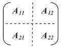
Where A₁₁ and A₂₂ are square matrices, and A₁₂ and A₂₁ are matrices or vectors.

Its inverse is

Where B11 and B₂₂ are square matrices, and B₁₂ and B₂₁ are matrices or vectors. They are of the same sizes as their corresponding A_ij.

Two solutions exist. The first solution is:

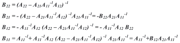
The second solution is

The matrices A11 - A₁₂A₂₂^-1 A₂₁ and A₂₂ - A₂₁A₁₁^-1A₁₂ are sometimes referred as the Schur complements (Haynsworth, 1968). In ordinary kriging, A₂₂ is the scalar 0. Therefore, its inverse does not exist and the first solution is used.