Geostatistical applications in petroleum reservoir modelling

 

 

R. Cao^I; Y. Zee Ma^II; E. Gomez^II

^IChina University of Petroleum, Beijing, China
^IISchlumberger, Denver, Colorado, USA

 

 

---

SYNOPSIS

Geostatistics was initially developed in the mining sector, but has been extended to other geoscience applications, including forestry, environmental science, soil science, and petroleum science and engineering. This paper presents methods, workflows, and pitfalls in using geostatistics for hydrocarbon resource modelling and evaluation. Examples are presented of indicator variogram analysis of categorical variables, lithofacies modelling by sequential indicator simulation and hierarchical workflow, porosity modelling by kriging and stochastic simulation, collocated cokriging for integrating seismic data, and collocated cosimulation for modelling porosity and permeability relationships. These methods together form a systematic approach that can be effectively used for modelling natural resources.

Keywords: facies modelling, propensity, multilevel or hierarchical modeling, objectbased modeling, collocated cosimulation, porosity, permeability.

---

 

 

Introduction

Although geostatistics was initially developed for mining resource evaluation (Krige, 1951; Matheron, 1963; Journel and Huijbregts, 1978), it has been used quite extensively in the petroleum industry in the past two to three decades. Geostatistical analysis and geological modelling have been commonly employed for hydrocarbon characterization. The success of geostatistics in geoscience applications rests upon the spatial descriptions of geological phenomena, from characterizing rock continuities using variograms (Jones and Ma, 2001) to three-dimensional (3D) representations of natural phenomena (Deutsch and Journel 1992; Ma et al., 2009).

Geostatistical methods for building geological models all make use of the variogram. The variogram describes the degree of discontinuity of a variable as a function of lag distance and direction. For a categorical variable such as facies, the variogram describes the size of geological objects (Jones and Ma, 2001). In hydrocarbon resource evaluation, facies are an intermediate-scale rock property as they govern petrophysical properties and fluid flow. This paper discusses the main characteristics of a lithofacies indicator variogram, and presents methods for modelling lithofacies, including sequential indicator simulation that integrates propensity analysis of descriptive geology, hierarchical facies, or lithofacies modelling workflows.

Reservoir models of continuous properties in hydrocarbon resource evaluation generally include porosity, fluid saturations, and permeability. This paper briefly discusses porosity modelling by using kriging and sequential Gaussian simulation, and permeability modelling by using collocated co-simulation. Based on the scale of subsurface heterogeneities, hierarchical modelling frameworks are presented not only for a two-step facies-lithofacies modelling workflow, but also for dealing with the more general multilevel modelling methodology, from the categorical variable of facies to continuous variables of porosity and permeability.

 

Facies and lithofacies modelling

Facies and lithofacies are discrete variables in which the rock property describes categories of the rock quality (Ma, 2011). An indicator variable represents a binary state with two possible outcomes: presence or absence. For three or more lithofacies, the indicator variable may be defined in terms of one lithofacies and all the others combined to indicate the absence of that selected lithofacies.

Indicator variogram

Most indicator variograms show the second-order stationarity with a definable plateau (Jones and Ma, 2001). The lithofacies variogram observed across stratigraphic formations is commonly strongly cyclical with lag distance. This has been termed a holeeffect variogram in geostatistics (Ma and Jones, 2001). Cyclicity and amplitudes in hole-effect variograms are strongly affected by the relative abundance of each lithofacies and by the means and standard deviations of the sizes of lithofacies objects (e.g. sandstone and shale bodies).

Sample density is very important for accurately describing an experimental variogram (Ma et al., 2009). In a reservoir with a low sandstone fraction, if individual sandstone or other lithofacies bodies are sampled densely (e.g. several data samples for each sand body), the experimental variogram will likely show spatial correlations and possibly a certain degree of cyclicity. However, if individual lithofacies bodies are sampled with only one observation each, the indicator variogram will appear with a strong nugget effect. This is consistent with the notion that geology is by no means random, but that sparse sampling can make it appear random.

Consider an experimental horizontal variogram generated while only a few wells have been drilled in the area. The closest spacing of the wells may be so great that a variogram cannot be determined for short lag distances. For instance, if the object size varies substantially for one lithofacies, the variability may override any signal that the periodic stratigraphy may carry. If the experimental variogram is calculated isotropically or with a wide tolerance around a specified direction, non-isotropic bodies (e.g. channels) will produce variograms with a mixture of spatial continuities.

For applications, an experimental variogram is typically fitted to a theoretical model. The spherical and exponential models, possibly with a partial nugget effect, are most commonly used in practice. These models imply monotonically increasing variance with increasing lag distance.

Sequential indicator simulation

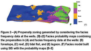
Sequential indicator simulation (SIS) is one of the most commonly used methods to model lithofacies because of its capabilities in integrating various data. In particular, lithofacies probability maps or volumes can be used to constrain the positioning of the geological objects in a SIS model. As a matter of fact, because of the complexity of depositional history, a geological process is simultaneously indeterministic and causal. Such a phenomenon can be described by the propensity, which enables quantitative integration of descriptive geology with lithofacies frequency data at wells (Ma, 2009). Such integration can produce lithofacies probabilities that convey the descriptive geology, and at the same time honour the available data. Subsequently, these lithofacies probabilities can be used to constrain stochastic modelling for building realistic geological models. The boundaries in the propensity zoning are often interpretive, in which case the geologist can incorporate the conceptual depositional model.

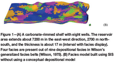
When no probability is used for conditioning, the lithofacies model is driven only by the indictor variogram and data from the wells. As a result of the scarcity of the data, the facies objects are often distributed unrealistically randomly, especially in the areas of no control points. In the example shown in Figure 1A, reef facies should occur only in the eastern rim of the shelf, but the model generates the reef facies everywhere (Figure 1B).

 

 

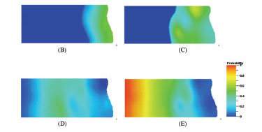
By integrating the propensity analysis (Figure 2A) based on the conceptual depositional model, the facies probability maps were generated (Figures 2B to 2E). The facies model constrained by these probability maps shows most reef facies in the east of the area (Figure 2F). The propensity influence is obvious in the model.

 

 

Hierarchical facies modelling

Apart from SIS, other techniques for modelling facies include object-based modelling (OBM, see e.g., Ma et al. 2011), Boolean, and truncated Gaussian methods (Deutsch and Journel, 1992; Falivene et al., 2006). All these categorical modelling techniques can be hierarchized in two or more levels for multilevel facies modelling. For example, facies may be first modelled using fluvial OBM or the truncated Gaussian method, and then modelled again using SIS based on the model already constructed. This is because the OBM and truncated Gaussian methods generally produce larger facies objects in the model, and SIS can be further used to model small-scale heterogeneities. OBM is suitable for clear shape definitions of geological features such as channels and bars. The truncated Gaussian method is suitable when the order of the facies is clearly definable.

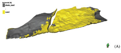
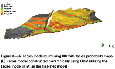
The workflow of modelling lithofacies by SIS following a truncated Gaussian modelling or OBM has been applied to a number of hydrocarbon field development case studies, including carbonate ramps and shallow marine depositional environments. Here, an example of constructing a facies model using OBM based on the model constructed by SIS is presented. A facies model of sand-shale (Figure 3A) was first built using SIS with facies probability maps. An OBM method was then used to generate channels with splays (Figure 3B). Splays occurs on the edges of the channels, but are not invariably present. Notice that channels erode both previously deposited shale and sand.

 

 

Kriging and stochastic simulation of porosity

Porosity is one of the most important petrophysical variables in hydrocarbon resource characterization, as it describes the subsurface pore space available for fluid storage. Geostatistical methods for modelling porosity include kriging and sequential Gaussian simulation (SGS). Kriging generally produces smoother results, as the variance of the kriging model is commonly smaller than the variance of the data used in the kriging. SGS can be considered to be a two-step modelling workflow that performs a stochastic simulation based on kriging results. Sometimes, cokriging or cosimulation can be used when more densely sampled seismic data is available and can be calibrated with porosity.

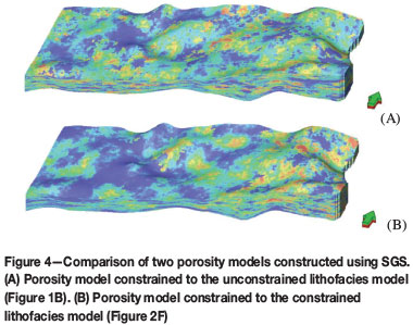
In addition, the lithofacies model is often used to constrain the spatial distribution of porosity using SGS, because in the hierarchy of subsurface heterogeneities, depositional facies govern spatial and frequency characteristics of porosity to a large extent. Even though porosity can still be quite variable within each fades, the porosity statistics by fades generally exhibit less variation (Ma et al, 2008). Figure 4 compares two porosity models constructed with the two different lithofacies models presented earlier (Figure 2).

 

 

Collocated cokriging and collocated cosimulation

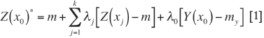
Collocated cokriging is a simplified version of cokriging (Xu et al, 1992). Instead of using a number of data points from the secondary variables, collocated cokriging uses only one data point that is collocated (i.e. at the same position) with the estimation point of the primary variable. Thus the estimator by collocated cokriging is such that:

where

m is the mean of the primary variable

λ_j are the weights of the data points of the primary variable

λ₀ is the weight of the collocated data point of the secondary variable

m_y is the mean of the secondary variable

Y(x₀) is the collocated secondary variable.

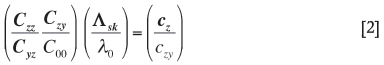
The simple kriging solution to Equation [1] is a linear system of equations obtained by the least-square method that minimizes the estimation error. That is, in a block matrix form:

where

C_ZZ represents the sample covariance matrix

C_zy' or its transpose, c_yz is the vector of covariances between each of the data points in the primary variable and the collocated data point of the secondary variable

C₀₀ is the variance of the secondary variable (equal to 1 after normalization)

A_sk is the vector of the simple kriging weights for the primary variable

λ₀ is the weight for the collocated data point of the secondary variable

c_z is the vector of covariances between each of the data points and the estimation point of the primary variable

C_zy is the covariance between the primary and secondary variables.

Special cases:

(1) When the collocated secondary variable is not used, the method is reduced to simple kriging

(2) When there is no sample data in the kriging neighborhood, collocated cokriging uses the sole data point of the secondary variable at the location, and becomes the linear regression. Indeed, k₀ is obtained as the correlation coefficient between the two variables (scaled by their ratio of standard deviations), which is the solution of the linear regression

(3) An advantage of collocated cokriging compared to linear regression is that it has the exactitude property, inherited from all the kriging methods, while linear regression does not. That is, it honours all the sample data. The proof is quite straightforward. Making one of the known points in Equations [1] and [2] the estimation point will lead to that point having a weight equal to 1 while all the other weights become zero.

Collocated cosimulation is somewhat similar to sequential Gaussian simulation, except that their kriging estimation equations are slightly different (see Equations [1] and [2]). It can also be formulated as the summation of an estimation and a simulated error.

It is noteworthy that an (auto-) covariance function is symmetrical about the origin (zero lag distance), but a cross-covariance function is not necessarily symmetrical. In such a case, cokriging cannot be simplified to collocated cokriging because the delay effect (see e.g. Papoulis, 1965) in correlation between the primary and secondary variables cannot be easily conveyed into the auto-covariance function. Moreover, even if the cross-covariance is symmetrical, there are some important approximations in reducing cokriging to a collocated cokriging (Deutsch and Journel, 1992). Theoretically, only some special cases verify the assumptions (Rivoirard, 2001). In practice, the simplification in collocated cokriging and co-simulation make these methods very useful in honouring the relationships between two variables.

Collocated cokriging can be quite effective in integrating seismic data into petrophysical property models (Xu et al., 1992). Collocated cosimulation is generally more useful for modeling permeability as it can honour the porosity-permeability relationship, often termed the phi-K relationship. An example of modelling the phi-K relationship is discussed below in comparison to linear regression.

The phi-K relationship in the data is often a clouded nonlinear correlation (Figure 5A). Imposing a linear transform between the porosity and logarithmetic permeability can significantly distort the frequency statistics of the permeability. In fact, the difference in frequency distribution between the permeability model generated using a standard linear regression and the well log data is commonly striking, as shown by the example in Figure 5B. The phi-K transform, in which the logarithm of permeability is estimated from the porosity using a linear transform, reduces the permeability because the exponential of the mean is smaller than the mean of the exponential (Delfiner, 2007). This effect of reduction can be easily seen by comparing the frequency distribution of the permeability from the linear regression to the original frequency distribution of the data. Indeed, a linear transform creates more low permeability values and skews the histogram toward the lower permeability values (Figure 5B).

Instead of using a phi-K transform or cloud transform, collocated cosimulation or 'cocosim' (Ma et al., 2008) can be used to honour the relationship between the permeability and porosity. The histogram of the permeability model using cocosim closely matches the histogram of the well log permeability data (Figure 5C). Besides avoiding the bias introduced in a phi-K transform (Ma, 2010), there are other advantages in using cocosim, including the 3D porosity model constraining the 3D permeability model, and honouring the data at the well locations.

 

Conclusion

In 3D modelling of subsurface processes, there is commonly a significant lack of hard data. To generalize the data to a 3D model, critical inferences must be made. The quality and accuracy of the model depend on not only the quality and quantity of data, but also how the inference is drawn and made. It is often said that 'garbage in, garbage out'. However, it should be noted that the 'data in' does not necessarily mean a good model will result; it can still result in 'garbage out' due to erroneous inference from the data to the model. Geostatistical methods provide tools for better inference from limited data in constructing a 3D reservoir model. These include incorporation of depositional interpretation using propensity analysis, variogram analysis, and the hierarchical modelling framework.

Propensity analysis can help the transition from qualitative description to quantitative analysis, bridge the gap between the descriptive geology and quantitative modelling, and provides useful constraints to condition the facies model to be geologically realistic. Variogram analysis can help characterize the continuity of rock properties, including geological object size and anisotropy. A broad hierarchical modelling workflow is an efficient way of modelling multi-scale subsurface heterogeneities, from large-scale structural and stratigraphic heterogeneities, to intermediate-scale facies heterogeneities, to smaller-scale petrophysical properties. Furthermore, some discrete variables in one category of a broad hierarchical workflow, such as facies, can be hierarchically modelled with two or more levels of modelling by different methods. An example of combining object-based modeling and SIS was given in this paper.

Geostatistical models of discrete lithofacies variables are important because of their use in constraining porosity and permeability models. Collocated cosimulation is an effective way to model porosity-permeability relationship while honouring the known permeability data and constraining the permeability model to the previously generated porosity model.

 

References

Bashore, W.M., Araktingi, U.G., Levy, M., and Schweller, W.J. 1994. Importance of a geological framework and seismic data integration for reservoir modeling and subsequent fluid-flow predictions. Stochastic Modeling and Geostatistics. Yarus, J.M. and Chambers, R.L. (eds.). American Association of Petroleum Geologists, Tulsa, OK. pp. 159-175.         [ Links ]

Caers, J. and Zhang, T. 2004, Multiple-point geostatistics: a quantitative vehicle for integrating geologic analogs into multiple reservoir models. AAPG Memoir 80. American Association of Petroleum Geologists, Tulsa, OK. pp. 383-394.         [ Links ]

Chiles, J-P. and Delfiner, P. 1999. Geostatistics: Modeling Spatial Uncertainty. John Wiley & Sons, New York. 695 pp.         [ Links ]

Delfiner, P. 2007. Three pitfalls of phi-K transforms. SPE Formation Evaluation and Engineering, Dec. 2007. pp. 609-617.         [ Links ]

Deutsch, C.V. and Journel, A.G. 1992, Geostatistical Software Library and User's Guide. Oxford University Press. 340 pp.         [ Links ]

Falivene, O., Arbues, P., Gardiner, A., Pickup, G., Munoz, J.A., and Cabrera, L. 2006. Best practice stochastic facies modeling from a channel-fill turbidite sandstone analog. AAPG Bulletin, vol. 90, no. 7. pp. 1003-1029.         [ Links ]

Jones, T.A. and Ma, Y.Z. 2001. Geologic characteristics of hole-effect variograms calculated from lithology-indicator variables. Mathematical Geology, vol. 33, no. 5. pp. 615-629.         [ Links ]

Journel, A. 1983. Nonparametric estimation of spatial distribution. Mathematical Geology, vol. 15, no. 3. pp. 445-468.         [ Links ]

Journel, A.G. and Huijbregts, C.J. 1978. Mining Geostatistics. Academic Press, New York. 600 pp.         [ Links ]

Krige, D.G. 1951, A statistical approach to some basic mine valuation problems in the Witwatersrand. Journal of the Chemical, Metallurgy, and Mining Society of South Africa, vol. 52. pp. 119-139.         [ Links ]

Ma, Y.Z. 2009. Propensity and probability in depositional facies analysis and modeling. Mathematical Geosciences, vol. 41. pp. 737-760. doi: 10.1007/s11004-009-9239-z.         [ Links ]

Ma, Y.Z. 2010. Error types in reservoir characterization and management. Jourmal of Petroleum Science and Engineering,, vol. 72, no. 3-4. pp. 290-301. doi: 10.1016/j.petrol.2010.03.030.         [ Links ]

Ma, Y.Z. 2011, Lithofacies clustering using principal component analysis and neural network: application to wireline logs. Mathematical Geosciences, vol. 43, no.4. pp. 401-419.         [ Links ]

Ma, Y.Z., Gomez, E., Young, T.L., Cox, D.L., Luneau, B., and Iwere, F. 2011. Integrated reservoir modeling of a Pinedale tight-gas reservoir in the Greater Green River Basin, Wyoming. Uncertainty Analysis and Reservoir Modeling. Ma, Y.Z. and LaPointe, P. (eds.). AAPGMemoir 96. American Association of Petroleum Geologists, Tulsa, OK.         [ Links ]

Ma, Y.Z., Seto, A., and Gomez, E. 2009, Depositional facies analysis and modeling of Judy Creek reef complex of the Late Devonian Swan Hills, Alberta, Canada. AAPG Bulletin, vol. 93, no. 9. pp. 1235-1256. doi: 10.1306/05220908103.         [ Links ]

Ma, Y.Z., Seto A., and Gomez, E. 2008. Frequentist meets spatialist: a marriage made in reservoir characterization and modeling. SPE 115836, Society of Petroleum Engineers, Annual Technical Conference and Exhibition. SPE, Denver, CO.         [ Links ]

Ma, Y.Z. and Jones, T.A. 2001. Modeling hole-effect variograms of lithology-indicator variables: Mathematical Geology, vol. 33, no. 5. pp. 631-648.         [ Links ]

Matheron, G. 1963, Principles of geostatistics, Economic Geology, vol. 58. pp. 1246-1266.         [ Links ]

Moore, C.H. 2001. Carbonate Reservoirs: Porosity Evolution and Diagenesis in a Sequence Stratigraphic Framework. Elsevier, Amsterdam. 444 pp.         [ Links ]

Papoulis, A. 1965. Probability, Random Variables and Stochastic Processes. McGraw-Hill, New York. 583 pp.         [ Links ]

Popper, K.R. 1995. A World of Propensities. Thoemmes, Bristol (reprinted). 51 pp.         [ Links ]

Rivoirard, J. 2001. Which models for collocated cokriging? Mathematical Geology, vol. 33, no. 2. pp. 117-131.         [ Links ]

Wilson, J.L. 1975. Carbonate Facies in Geologic History. Springer Verlag, New York. 471 pp.         [ Links ]

Xu, W., Tran, T.T., Srivastava, R.M., and Journel, A.G. 1992. Integrating seismic data in reservoir modeling: the collocated cokriging alternative. SPE 24742. Society of Petroleum Engineers, 67th Annual Technical Conference and Exhibition. SPE, Denver, CO. pp. 833-842.         [ Links ]