Investigating 'optimal' kriging variance estimation using an analytic and a bootstrap approach

 

 

C. Thiart^I; M.Z. Ngwenya^II; and L.M. Haines^I

^IDepartment of Statistical Sciences, University of Cape Town, South Africa
^IIBiometry Unit, Agricultural Research Council, Stellenbosch, South Africa

 

 

---

SYNOPSIS

Kriging is an interpolation technique for predicting unobserved responses at target locations from observed responses at specified locations. Kriging predictors are best linear unbiased predictors (BLUPs) and the precision of the BLUP is assessed by the mean square prediction error (MSPE), commonly known as the kriging variance. Both the BLUP and the MSPE depend on the covariance function describing the spatial correlation between locations and on specific parameters. The parameters are usually treated as known, whereas in practice they invariably have to be estimated and the empirical BLUP (that is, the EBLUP) so obtained. The empirical or estimated mean square prediction error (EMSPE), or the so called 'plug-in' kriging variance estimator, underestimates the true kriging variance of the EBLUP, at least in general. In this paper five estimators for the kriging variance of the EBLUP are considered and compared by means of a simulation study in which a Gaussian distribution for the responses, an exponential structure for the covariance function, and three levels of spatial correlation - weak, moderate, and strong - are adopted. The Prasad-Rao estimator obtained using restricted or residual maximum likelihood (REML) is recommended for moderate and strong spatial correlation and the Kacker-Harville estimator for weak correlation in the random fields.

Keywords: kriging, covariance parameters, mean square prediction error.

---

 

 

Introduction

The problem of accommodating correlation between observations made at different locations permeates design, analysis, and prediction for spatial data. In two seminal papers, Krige formulated a statistical model for such data, which comprises a deterministic component reflecting the underlying trends and an error component capturing correlations between observations taken at separate locations (Krige, 1951), and invoked his model to obtain predictions at unobserved locations (Krige, 1962). Krige's work provided the basis for best linear unbiased prediction within the context of spatial data and was formalized more rigidly and mathematically by Matheron (1963). An excellent overview of the historical development of the methodology, broadly referred to as kriging, is provided by Cressie (1990).

The kriging approach has been adapted seamlessly to accommodate more modern statistical practice and is used extensively in a vast range of areas. A particular problem, that of using best linear unbiased prediction to predict a response at an unobserved location when the parameters describing the correlation structure between locations are unknown is, however, not fully resolved. To be specific, an obvious solution to this problem is to 'plug' an available estimate of the parameters into the expression for the predictor with parameters known. Unfortunately, the distribution of the resultant predictor, termed the empirical best linear unbiased predictor or EBLUP, is intractable, and more particularly the mean square prediction error associated with the EBLUP cannot be expressed analytically.

In the present study, five approaches to approximating the mean square prediction error of the EBLUP, the 'plug-in', those of Kacker and Harville (1984) and Prasad and Rao (1990), and two taken from den Hertog et al. (2006) and based on bootstrapping, are introduced and compared using a simulation study that accommodates weak, moderate, and strong spatial correlation. The paper is organized as follows. Basic notions and formulae underpinning the methodology are presented first. The simulation study is then described, and the attendant results summarized. Finally, some broad conclusions and pointers for further research are given.

 

Preliminaries

Kriging basics

Suppose that observations are made on an attribute Z at the n spatial locations xi, i = 1, ..., n, in a designated geographic region D. Let Z (xg) denote the observed response at a generic location x_g where x_gDR² and let Z(x) where x = (x1, ... , xn) denote the n W 1 vector of responses at the n locations. Suppose further that interest centres on predicting the response Z(x0) at a location x0 in D. Then it is usual to obtain such a predicted value by introducing a weighted sum of the observations of the form

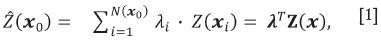
where λi is the weight associated with the ith observation Z(xt)with , λis the n xl vector and N(x0) is the number of points in a search neighbourhood around the prediction location x0.

Now, assuming second-order stationarity, the kriging model can be formulated as

where F(x) is an n W (k + 1) matrix with rows which usually depend on the spatial coordinates alone and/or other explanatory variables, β is a vector of k + 1 unknown parameters, and e (x) is an n + 1 vector of error terms with mean 0 and variance-covariance matrix Σ (θ). The covariance between any two points is taken here to be a function of the Euclidean distance between the two points and the vector of parameters θ =(θ0, θ1,θ2), corresponding, in order, to the nugget, the partial sill, and the range. Other functions for the covariance between points, such as the exponential and the Matirn, which depend on more or fewer parameters, can also be invoked (Diggle and Ribeiro, 2007). The covariance between any two points, xt and xj is denoted as Cov[Z(xi), Z(xj)] = C(xi - xj; θ) and for i, j = 1,..., n are the elements of the variance-covariance matrix.

The best linear unbiased predictor (BLUP) at location x₀ under the kriging model in Equation [2] is obtained by minimizing the mean square prediction error, E[λ^TZ(x) -Z(x₀)]², with respect to the weights λunder the condition of unbiasedness, that is E[(x₀)] = Z(x₀). Thus, assuming the parameter θis known, the kriging weight vector λis given by

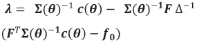
where c(θ) is the n W1 vector (C(x₀-x₁; θ), ... , (C(x₀-x_n; θ)), Δ = F^TΣ(θ)^-1F and f₀ = F^Tλ. It then follows that the BLUP at x0 is given by

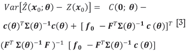
and its mean square prediction error, denoted MSPE and termed the kriging variance, by

where is the generalized least squares (GLS) estimator of β, that is

In practice, however, the parameters θ = (θ0, θ1, θ2) are rarely known and must be estimated. Early studies adopted least squares estimators of θ based on fitting appropriate nonlinear models to the semivariogram data. However, a more modern approach involves maximizing the log-likelihood or the restricted log-likelihood with respect to β and θ to give the maximum likelihood estimator (MLE), MLE, or the restricted maximum likelihood (REML) estimator, MLE, of θ respectively. The kriging predictor at the location x0 is then obtained by 'plugging' an estimate of θ, denoted generically , into the expression for the BLUP to give the 'empirical' BLUP, termed the EBLUP, as

.

In the same spirit, the kriging variance or MSPE of the predictor at x0 can be estimated by plugging into the expression for the MSPE with θknown, that is into Equation [3], to give the 'empirical' MSPE, denoted EMSPE and more commonly referred to as the plug-in kriging variance estimator.

Kriging variance estimators

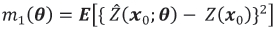
It is well known that the plug-in estimator of the kriging variance underpredicts the MSPE of the EBLUP, at least in general (Zimmerman and Cressie, 1992, den Hertog et al. 2006). More specifically, the MSPE with θ and Σ(θ) known is given in Equation [3] and can be expressed succinctly as

.

Thus, for θ unknown, the EMSPE, that is the plug-in kriging variance, is given by m1(). Strictly, however, the mean square prediction error associated with the EBLUP is given by

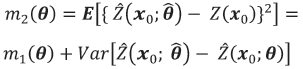
where the trailing term in the second equality is algebraically intractable and therefore m2() cannot be evaluated. A number of approaches, both algebraic and computational, to the construction of estimators of the EBLUP kriging variance, which are approximate and which to some extent redress the negative bias in the EMSPE, have been reported. In this study the properties of four such estimators, namely the Kacker-Harville estimator, the Prasad-Rao estimator, and two bootstrap estimators, are investigated. These estimators are summarized as follows.

Kacker and Harville (1984) used a Taylor series expansion of the trailing term in m2(θ) to derive an estimator of the EBLUP kriging variance, albeit approximate, as

where

.

In practice can be plugged into the terms m1 (θ)and Α (θ) of Equation [4] and the term B (θ), which is the mean square error of and is unknown, can be approximated by the inverse of the observed Fisher information matrix for θ, that is the inverse of the Hessian H(). Thus the Kacker-Harville estimator can be evaluated as

but, since this is essentially a plug-in estimator, it still remains negatively biased. To redress this bias, Prasad and Rao (1990) invoked some intricate theory to develop a further correction to m2(θ) and, based on their results, introduced an estimator which approximates the MSE of the EBLUP as

Both the Kacker-Harville and the Prasad-Rao estimators reduce the negative bias of the plug-in kriging variance, but the improvement depends on sample size, spatial autocorrelation, Gaussian assumptions, an unbiased estimate of θ, and on the assumption that the covariance function is linear in the elements of θ(Prasad and Rao, 1990; Harville and Jeske, 1992; Zimmerman and Cressie, 1992). However, the latter assumption is clearly not valid for a range of widely used covariance models, such as the Gaussian, the exponential, the spherical, and the Matirn. This observation prompted Wang and Wall (2003) to suggest bootstrapping as an alternative method for estimating the MSPE of the EBLUP.

Two bootstrap estimators of m2(θ) are investigated in the present study. Specifically, suppose that observations Z(x) at the n locations, x1, ..., xn, are taken from a Gaussian random field and that predictors at m new or test locations, x01, ... , x0m, are required. The MLE or REML estimators of β and θ, denoted and respectively, can immediately be obtained from the data and, following den Hertog et al. (2006), bootstrap procedures based on the estimated distribution Z(x) ~ G (F, Σ()) can then be implemented.

The bootstrap estimator of the MSPE of the EBLUP based on the assumption of a joint or unconditional Gaussian distribution for the responses at the observed and the test locations, termed the unconditional bootstrap estimator (UBE) and denoted , is introduced here and can be obtained by implementing the following algorithm.

Unconditional bootstrap estimation

1. Sample from G (F, Σ()) at the observed locations x1, ... , xn and at the test locations x01, ... , x0m simultaneously

2. Use the bootstrap sample at the n observed locations to fit a kriging model and use this fitted model to compute predictions at the m test locations x01, ... , x0m

3. Calculate the squared prediction error at each test point

4. Repeat steps 1 to 3 B times. Then compute the unconditional bootstrap estimate of the MSPE, that is m2(UBE)() , at each test point. Stop.

An alternative bootstrap estimator to the UBE, termed the conditional bootstrap estimator (CBE) and denoted m2(CBE)() , is based on the fact that the conditional distribution of the responses Z(x0) at the test locations, x01,..., x0m, given observations Z(x) at the n locations, x1... , xn under a Gaussian assumption is well known. Specifically,

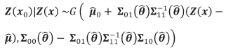
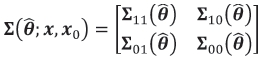
where the vectors and with evaluated at , are the vectors of estimated means at the n observed and the m test locations respectively and the variance matrix for x = (x1... , xn) and x01i... , x0m, partitioned conformably with these vectors, is given by

.

The conditional bootstrap estimator is also introduced in the present study and can be obtained by implementing the following algorithm.

Conditional bootstrap estimation

1. Use the kriging model, fitted to the observations Z(x) to make predictions at the m test locations x01i..., x0m

2. Take a bootstrap sample at the test locations x01.,..., x0m conditional on the observations Z(x), that is, sample from the conditional distribution Z(x0)|Z(x)

3. Calculate the squared differences of the predictions and the bootstrap realizations obtained from steps 1 and 2 respectively

4. Repeat steps 2 and 3 B times. Then compute the conditional bootstrap estimate of the MSPE, that is, m2(CBE) () , at each test point. Stop.

 

Simulation study

In order to investigate the performance of the five estimators for the MSPE of the EBLUP introduced in this paper, namely the plug-in, the Kacker-Harville, the Prasad-Rao, the unconditional bootstrap, and the conditional bootstrap estimators, a simulation study incorporating conditions of spatial correlation specified by three Gaussian random fields was undertaken (Ngwenya, 2009).

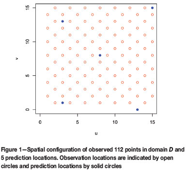
Settings for the simulations are summarized as follows. The observed locations were taken as a regular grid of 112 points in a square domain D = [0,15] x [10,15] and are specified by the set

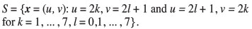
In addition, a set of five points, {x01 ,... , x05} = {(3,1),(13,0),(8,8),(3,13),(15,15)} within the domain D, was chosen to specify the prediction locations (Figure 1). The five prediction points were located so as to enable the effective study of location and data configuration on the various m2(θ) estimators. We have chosen a point in the middle of the grid, one inside the grid but close to the edge of the domain D, two on the edge of the grid, and one outside the grid but still in D.

 

 

An ordinary kriging model with F(x) = 1 and a Gaussian distribution for the error terms, namely

,

was adopted. More specifically, the regression parameter βwas taken to be zero, thus defining a simple kriging model, and an exponential covariance structure

where h denotes the Euclidean distance between the locations xi and xj, θ1 the nugget, θ2 the partial sill, and θ3 the range, as adopted. Fixed values of θ1 = 0.25 and θ2 = 1 were taken and three values for the range, namely θ3 = 1.5, 2.5, and 4.2 corresponding to weak, moderate, and strong spatial correlations respectively, were introduced. Thus three datasets or random fields, denoted Z1, Z2 and Z3, with increasing spatial correlation were created.

It is sensible to compare each of the five estimators of the MSPE of the EBLUP introduced in this study with the true value, m2(θ). As noted earlier, no analytical expression for m2(θ) is available. However Monte Carlo simulation to approximate the true value m2(θ) to a chosen degree of accuracy can readily be performed. The procedure is summarized as follows.

Monte Carlo procedure to approximate m2(θ)

1. Set r = 1

2. Generate a spatial process over the grid of observation and prediction locations using the true values of the parameters β and θ

3. For the rth realization fit a kriging model by using the data at the observation locations to obtain estimates r of β and r of θ

4. Calculate 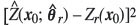, the squared difference between the predicted value and the observed value Zr(xo) at each of the prediction locations, x0

5. Repeat steps 2 to 4, updating r to r + 1, R times and then compute the average squared differences between the predicted and simulated values as

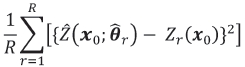
for each of the prediction locations, x0. Stop.

A pilot study to determine the number of simulations R that gives m2(θ) to an accuracy of at least ±0.0001 for each of the three random fields, Z1, Z2, and Z3, was performed. A maximum value of R = 250 000 for the full Monte Carlo simulations was found and used in all cases.

The plug-in, the Kacker-Harville, and the Prasad-Rao estimators of the MSPE of the EBLUP at the m = 5 prediction locations for each of the random fields Z1, Z2, and Z3, were based on 1000 realizations at the observation locations. Specifically, for each realization the MLE and REML estimates of θ, denoted generically as , were found and plugged into the appropriate expressions. The resultant estimates were then averaged over the 1000 realizations to give the estimators m1() , m2(KH)( ₎ and m_2(PR)() to a degree of accuracy determined by the number of simulations. The bootstrap estimators were based on B = 1000 bootstrap iterations for each of the 1000 realizations of the observed and, in the case of the unconditional bootstrap estimator, the observed and the prediction locations. The unconditional bootstrap method is computationally expensive since 1000 W 1000 W 2 (MLE and REML) = 200 000 kriging models had to be fitted to the simulated data. This consideration limited the number of realizations.

 

Results

The values the MSPE of the BLUP, m1(θ), the MSPE of the EBLUP, m2(θ), and the EMSPE m1() together with the values of the four alternative kriging variance estimators, namely m2(KH)() , m2(PR)() , m2(UBE)() and m2(CBE)() , under both MLE and REML estimation of the covariance parameters, were computed at each prediction location across the three random fields, Z1, Z2, and Z3. The R programming language (R Development Core Team, 2012) was used to calculate these values and the results are tabulated in Ngwenya (2009). For conciseness, only the relative biases in the estimators of the MSPE of the EBLUP are presented here, with relative bias defined to be

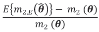
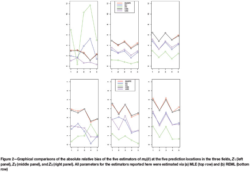
where m2,E() , is a generic estimator of m2(θ). Specifically, the relative biases under MLE and REML estimation of the covariance parameters θ are summarized in Table I(a) and I(b) together with m2(θ) values obtained by the Monte Carlo procedure. In addition, the absolute values of the percentage relative biases are represented diagrammatically in Figures 2(a) and 2(b) respectively.

Certain features of the relative biases in the MSPEs of the EBLUP are worth noting. In particular, the performance of the conditional bootstrap estimator m2(CBE)() is almost indistinguishable from that of the plug-in estimator m1() under both MLE and REML estimation of θ and at each point across the three random fields. These estimators seriously underestimate m2(θ), with the degree of underestimation increasing with an increase in the spatial correlation exhibited by the random fields.

The Kacker-Harville and unconditional bootstrap estimators, m2(KH)() and m2(UBE)() respectively, also exhibit very similar behaviour, but only when the spatial correlation is moderate to strong. It is interesting to note here that Zimmerman (2006), in simulation studies on optimal network designs, found that design criteria based on m2(KH)() and m2(UBE)() lead to similar designs. However, when the spatial correlation is weak, m2(KH)() has a propensity to lead to overestimates of m2(θ), while m2(UBE)() exhibits a high degree of accuracy, with an absolute relative bias as small as 0.3% at the prediction location (15, 15). In contrast, the estimators m2(KH)( _REML) and m_2(UBE)(REML) are more evenly matched when the spatial correlation is weak.

Values of m2(θ), at the points (3,1), (15,15), and (13,0), which lie at an edge, a corner, and outside of the area circum-scribed by the grid of observed locations, are greater than those for the prediction points (8,8) and (3,13), which are surrounded by observed locations. However it is also clear from the results summarized in Table I that this feature of the values of m2(θ) for the prediction points is not mirrored in the corresponding values of the absolute relative biases. Indeed, there seems to be no obvious relationship between these measures of bias and the location of the prediction points and the spatial configuration of the grid, in accord with the findings of Zimmerman and Cressie (1992).

The Prasad-Rao estimator m2(PR)() does not seem to exhibit behaviour that is very close to any of the other four estimators of the MSPE of the EBLUP investigated in this study. Specifically, when the spatial correlation is weak, the estimator exhibits a large positive bias of up to 11.7% with MLE and 2.3% with REML. This observation can be explained by the fact that, for weak spatial correlation, the large sample covariance matrix overestimates the variability in the parameter estimates , thereby inflating the trailing term in the expression for m2(PR)() (Abt, 1999). The same explanation can be given for the fact that m2(KH)() has a propensity to be positively biased when the spatial correlation is weak. In contrast, for moderate and strong spatial correlation, the Prasad-Rao estimator m2(PR)() exhibits the smallest absolute relative bias at all prediction locations when compared to the other four estimators of m2(θ) in accord with the findings of Zimmerman and Cressie (1992). In fact, the Prasad-Rao estimator performs well with both MLE and REML in these situations, with biases as small as 0.5% and 0.1% respectively, and is clearly to be preferred.

 

Conclusions

Some broad conclusions based on the simulation study are now drawn, but should be taken strictly within the context of that study. Thus the performance of all of the five estimators of the mean square prediction error examined here depend somewhat sensitively on the method of estimation, that is MLE or REML, and in most cases REML should be the desired choice. The plug-in estimator consistently underestimates the MSPE of the EBLUP, in accord with more general findings in the literature, and is clearly unsatisfactory. The Prasad-Rao estimator performs optimally for the random fields with moderate and strong spatial correlation but would seem to be erratic for the field with weak correlation. In the latter case the Kacker-Harville estimator is to be preferred overall. It is interesting to note that the absolute relative biases of the prediction points do not appear to be related in any meaningful way to the location of those points in the domain of the simulation experiment.

Empirical studies on the nature and performance of approximate estimators for the MSPE of the EBLUP based on simulation or real data can be construed as being endless. Clearly, therefore, there is scope for further theoretical research into constructing reliable and robust estimators of this MSPE. One such approach could involve third-, fourth-, and higher-order approximations of appropriate Taylor series expansions. However, such derivations are intricate and nontrivial and indeed are fraught with subtle problems.

 

Acknowledgments

The authors would like to thank the reviewers for their helpful comments. They would also like to thank the University of Cape Town and the National Research Foundation (NRF) of South Africa, grants (UID) 85518 and (UID) 85456, for financial support. Any opinion, finding, and conclusion or recommendation expressed in this material is that of the authors and the NRF does not accept liability in this regard.

 

References

Abt, M. 1999. Estimating the prediction mean squared error of a Gaussian stochastic process with exponential correlation structure. Scandinavian Journal of Statistics, vol. 26. pp. 563-578.         [ Links ]

Cressie, N. 1990. The origins of kriging. Mathematical Geology, vol. 22. pp. 239-252.         [ Links ]

Den Hertog, D., Kleijnen, J.P.C., and Siem A.Y.D. 2006. The correct kriging variance estimated by bootstrapping. Journal of the Operational Research Society, vol. 57. pp. 400-409.         [ Links ]

Diggle, P.J. and Ribeiro, P.J. 2007. Model-based Geostatistics. Springer, New York.         [ Links ]

Harville, D.A. and Jeske, D.R. 1992. Mean squared error of estimation or prediction under a general linear model. Journal of the American Statistical Association, vol. 87. pp. 724-731.         [ Links ]

Kacker, R.N. and Harville, D. 1984. Approximations for standard errors of estimators of fixed and random effect in mixed linear models. Journal of the American Statistical Association, vol. 79. pp. 853-862.         [ Links ]

Krige, D.G. 1951. A statistical approach to some basic mine valuation problems on the Witwatersrand. Journal of the Chemical, Metallurgical and Mining Society of South Africa, vol. 52. pp. 119-139.         [ Links ]

Krige, D.G. 1962. Effective pay limits for selective mining. Journal of the South African Institute of Mining and Metallurgy, vol. 62. pp. 345-363.         [ Links ]

Matheron, G. 1963. Principles of geostatistics. Economic Geology, vol. 58. pp. 1246-1266.         [ Links ]

Ngwenya, M.Z. 2009. Investigating 'Optimal' Kriging Variance Estimation: Analytic and Bootstrap Estimators. Master's thesis, University of Cape Town, South Africa.         [ Links ]

Prasad, N.G.N. and Rao, J.N.K. 1990. On the estimation of the mean square error of small area predictors. Journal of the American Statistical Association, vol. 85. pp. 163-171.         [ Links ]

R Developement Core Team. 2012. R: A Language and Environment for Statistical Computing. R Foundation for Statistical Computing, Vienna, Austria. ISBN 3-900051-07-0.         [ Links ]

Wang, F. and Wall, M.M. 2003. Incorporating parameter uncertainty into prediction intervals for spatial data modelled via parametric variogram. Journal of Agricultural, Biological and Environmental Statistics, vol. 8. pp. 296-309.         [ Links ]

Zimmerman, D.L. 2006. Optimal network design for spatial prediction, covariance parameter estimation, and empirical prediction. Environmetrics, vol. 17. pp. 635-652.         [ Links ]

Zimmerman, D.L. and Cressie, N. 1992. Mean squared prediction error in the spatial linear model with estimated covariance parameters. Annals of the Institute of Statistical Mathematics, vol. 44. pp. 27-43.         [ Links ]