Geostatistics: a common link between medical geography, mathematical geology, and medical geology

 

 

P. Goovaerts

BioMedware, Inc, Ann Arbor

 

 

---

SYNOPSIS

Since its development in the mining industry, geostatistics has emerged as the primary tool for spatial data analysis in various fields, ranging from earth and atmospheric sciences to agriculture, soil science, remote sensing, and more recently environmental exposure assessment. In the last few years, these tools have been tailored to the field of medical geography or spatial epidemiology, which is concerned with the study of spatial patterns of disease incidence and mortality and the identification of potential 'causes' of disease, such as environmental exposure, diet and unhealthy behaviours, economic or socio-demographic factors. On the other hand, medical geology is an emerging interdisciplinary scientific field studying the relationship between natural geological factors and their effects on human and animal health. This paper provides an introduction to the field of medical geology with an overview of geostatistical methods available for the analysis of geological and health data. Key concepts are illustrated using the mapping of groundwater arsenic concentration across eleven Michigan counties and the exploration of its relationship to the incidence of prostate cancer at the township level.

Keywords: geostatistics, medical geology, spatial epidemology, groundwater, arsenic.

---

 

 

Introduction

Etymologically, the term 'geostatistics' designates the statistical study of natural phenomena. The early developments of geostatistics in the 1950s and 1960s aimed to improve the evaluation of recoverable reserves in mineral deposits (Krige, 1951; Journel and Huijbregts, 1978). Its field of application expanded considerably to encompass nowadays most fields of geoscience (e.g. geology, geochemistry, geohydrology, soil science) and a vast array of disciplines that all deal with the analysis of space-time data, such as oceanography, hydrogeology, remote sensing, agriculture, and environmental sciences. The success of geostatistics resides in its ability to capitalize on the first law of geography, stating that 'Everything is related to everything else, but near things are more related than distant things' (Tobler, 1970). Indeed, one of the main characteristics of the aforementioned data types is their structured distribution in space and time, which reflects the impact of various factors (e.g. geology, weather, human activities, land cover) operating at different spatial and temporal scales. Geostatistical spatio-temporal models (Kyriakidis and Journel, 1999) provide a probabilistic framework for data analysis and predictions that build on the joint spatial and temporal dependence between observations.

The main steps of a typical geostatistical study are summarized in Figure 1 using the well-known Swiss Jura data-set (Goovaerts, 1997, 1999). Analysis of spatial data typically starts with a 'posting' of data values. For example, Figure 1 (top graph) shows the location of 259 soil samples where the concentrations of topsoil cadmium concentration were recorded. Most applications of geostatistics are concerned with the prediction of measured attributes at unsampled locations. Such interpolation or extrapolation is made possible by the existence of autocorrelation in the data, which can be quantified and modelled using the semivariogram. Various kriging techniques are then available to derive estimated attribute values and the corresponding prediction error variance at unsampled locations using information related to one or several attributes. An important contribution of geostatistics is the assessment of the uncertainty about the attribute values at any particular unsampled location (local uncertainty) as well as jointly over several locations (multiple-point or spatial uncertainty). Models of local uncertainty usually take the form of a map of the probability of exceeding critical values, such as regulatory thresholds in soil pollution. Spatial uncertainty is tackled through stochastic simulation that allows one to generate alternative models of the spatial distribution of attribute values that reproduce features of the data (e.g. histogram, semivariogram). Last but not least, this uncertainty assessment can be combined with expert knowledge for decision-making, such as delineation of contaminated areas where remedial measures should be taken or selection of locations for additional sampling.

 

 

Medical geography is defined as the branch of human geography concerned with the geographic aspects of health, disease, and health care (May, 1950). The idea that place and location can influence health is a very old and familiar concept in medical geography. One of the first demonstrations of the power of mapping and analysing health data was provided by Dr John Snow's study of the cholera epidemic that ravaged London in 1854. Using maps showing the locations of water pumps and the homes of people who died of cholera, Snow was able to deduce that one public pump was the source of the cholera outbreak (McLeod, 2000). Since then, the field of medical geography has come a long way, replacing paper maps with digital maps in what are now called geographic information systems (GIS). Similarly, descriptive speculation about disease has given place to scientific analysis of spatial patterns of disease, including hypothesis testing, multi-level modelling, regression, and multivariate analysis.

Recently, geostatistical techniques (semivariograms, kriging, stochastic simulation) have been tailored to the study of spatial patterns of disease incidence and mortality and the identification of potential 'causes' of disease, such as environmental exposure or socio-demographic factor (Waller and Gotway, 2004; Goovaerts, 2007, 2009). Once again, health outcomes, such as cancer mortality or incidence of late-stage diagnosis, tend to follow the first law of geography, and maps are used by public health officials to identify areas of excess (e.g. cancer clusters) and to guide surveillance and control activities, including consideration of health service needs and resource allocation for screening and diagnostic testing. Data available for human health studies falls within two main categories: individual-level data (e.g. location of patients and controls) or aggregated data (e.g. cancer rates recorded at county or ZIP code level); see example in Figure 2. Although none of these data-sets falls within the category of 'geostatistical data' as classically defined in the spatial statistics literature (Cressie, 1993), geostatistics offers a promising alternative to common methods for analysing spatial point processes and lattice data. One of the most challenging tasks in environmental epidemiology is the analysis and synthesis of data collected at different scales and over different spatial supports. For example, one might want to explore relationships between health outcomes aggregated to the ZIP code level, census-tract demographic covariates, and exposure data measured at a few point locations. Geostatistics provides a theoretical framework for performing the various types of changes of support, while providing a measure of the reliability of the predictions (Goovaerts, 2010, 2012).

 

 

'Hydrobiogeochemoepidemiopathoecology', a term coined by scientists as an alternative to the most common medical geology, is defined as the science dealing with the relationship between natural geological factors and health in humans and animal, and understanding the influence of ordinary environmental factors on the geographical distribution of such health problems (Selinus et al., 2005). Bowman et al. (2003) distinguished two branches of medical geology, depending on whether health problems are caused by the natural occurrence of elements in the geologic environment (e.g. ingestion of food grown in soils with element deficiency or toxicity) or the release of elements by natural hazards, such as earthquakes, volcanic eruptions, or landslides. Like medical geography, the first applications of medical geology can be traced back to the distant past. The Romans recognized potential health hazards related to mining, whereas the Chinese had noticed relationships between lung disease and rock crushing. According to Selinus (2004), one of the oldest documentations of medical geology was provided by Marco Polo, who reported in 1275 that his European horses were dying in the mountainous areas of China. The symptoms he described are consistent with poisoning by selenium, which is present in high natural concentrations in these areas.

Since then, there have been many examples of how geology impacts human and animal health, through both an excess (e.g. arsenic in drinking water and skin cancer, radon and lung cancer) or deficiency (e.g. iodine and goitre, soil minerals and poor growth of livestock) of naturally occurring chemical elements. In the 20th century, many map studies were published linking disease distribution to rock or soil types. For example, superimposing the map of incidence for podoconiosis (type of elephantiasis or leg swelling) on a geological map of East Africa revealed a correlation between this disease and the presence of red clays rich in alkali metals like sodium and potassium and associated with volcanic activity (Price, 1976). Finkelman et al. (2011) reported that lung cancer incidence and mortality in Ontario are highest in areas underlain by uranium-rich heavy clay and the Canadian Shield. The link between the fluoride geochemistry of water in an area and the occurrence of dental fluorosis is also a well-known relationship in medical geology (Dissanayake, 2005).

Because geostatistics is well established in mathematical geology and its application is growing in medical geography, it is natural to foresee a bright future for this discipline in the emerging field of medical geology. This paper provides a brief overview of geostatistical methods available for the analysis of environmental and aggregated health data, with an application to the mapping of prostate cancer incidence in Michigan and the exploration of its relationship to groundwater arsenic level.

 

Setting the problem

Arsenic (As) is one of the most toxic elements in our environment and is listed as the third most toxic substance, after lead and mercury in the US Toxic Substances and Disease Registry. Its adverse impact on human health can take many forms, including skin lesions, cardiovascular disease, hypertension, reproductive and neurological disorders, respiratory problems, and various types of cancer (e.g. skin, lung, liver, bladder, prostate, kidney). Sources of arsenic exposure vary from burning of arsenic-rich coal (China) and mining activities (Malaysia, Japan) to the ingestion of tainted food [e.g. rice) or water contaminated by natural sources such as bedrock containing arsenic (e.g. Bangladesh, India, Taiwan, Philippines, Mexico, Chile). Arsenic in drinking water is a major problem and has received much attention because of the large human population exposed and the extremely high concentrations (e.g. 600 to 700 lg/L) recorded in many instances. Few studies have, however, assessed the risks associated with exposure to low levels of arsenic (say < 50 lg/L) most commonly found in drinking water in the USA.

Elevated levels of naturally-occurring arsenic have been identified in regional patterns within the USA and are attributed to geochemistry, geology, climate, and glacial history (Welch et al., 2000). In the Michigan Thumb region, arsenopyrite (up to 7% As by weight) has been identified in the bedrock of the Marshall Sandstone aquifer, one of the region's most productive aquifers (Westjohn et al., 1998). The present case study explores the association between the incidence of prostate cancer and groundwater arsenic level for eleven Michigan counties displayed in Figure 3. Epidemiologic studies have suggested a possible association between exposure to inorganic arsenic and prostate cancer mortality, including a study of populations residing in Utah (Lewis et al., 1999). Unlike the Utah study no individual-level data is available here, which prohibits any exposure reconstruction (i.e. length of exposure is unknown in the absence of information on residential history) and the incorporation of important covariates, such as age, smoking, diet, heredity, or socio-economic status. Note that the objective of the case study is to illustrate the application of geostatistics in medical geology, and a thorough epidemiological study is beyond the scope of this paper.

 

 

The information available for this so-called ecological study (i.e. analysis of aggregated health outcomes) consist of: (1) 9 188 arsenic concentrations measured at 8 212 different private wells that were sampled between 1993 and 2002, (2) prostate cancer incidence recorded at the township level over the period 1985-2002, and (3) block-group population density that served as proxy for urbanization and use of regulated public water supply versus use of potentially contaminated private wells in rural areas. Figure 4A shows a close-up of these three data-sets in the northern part of the study area. This case study illustrates a common challenge in environmental epidemiology - that is, the analysis and synthesis of spatial data collected at different spatial scales and over different spatial supports. Exploring the relationships between these incompatible data-sets will require the estimation of all three variables over the same set of geographical units (i.e. townships here); see Figure 4B. Following the terminology in Gotway and Young (2007), this change of support (COS) will involve upscaling (spatial aggregation) for arsenic data and side-scaling, a term used to refer to the prediction of values on one set of spatial units from data on another set of overlapping spatial units, for population density.

 

 

Mapping arsenic content

This study will use the geostatistical model of the spatial distribution of groundwater arsenic concentrations that was described in details in Goovaerts et al. (2005). Only the most salient features will be presented here. The modelling was based on all 9 188 well data. The small magnitude of temporal variation relative to the variability in space or arising from measurement error, as well as the absence of temporal trend or seasonality, led us to ignore the temporal dimension in this study. Since this database contains arsenic measurements requested by homeowners, sampling is denser in areas where higher pollutant concentrations were initially reported. This preferential sampling was corrected using the cell-declustering technique (Deutsch and Journel, 1998), which calls for dividing the study area into rectangular cells; then each observation within a cell is assigned a weight inversely proportional to the number of data within that cell. These declustering weights were used, instead of equal weights, in the computation of summary statistics, leading to a mean and standard deviation of 10.97 and 15.22 lg/L, respectively.

Arsenic concentration was estimated at the nodes of a 500 m spacing grid using soft indicator kriging (Goovaerts, 1997) and 22 threshold values. Soft information was derived by a calibration of geological data, such as type of bedrock and unconsolidated deposits, and proximity of wells to the Marshall Sandstone suboutcrop, where the highest concentrations of arsenic were found. The choice of a non-parametric approach over lognormal or multigaussian kriging was motivated by:

1. The presence of 737 measurements below the detection limit. Unlike other techniques, indicator kriging does not require assigning a subjective value (e.g. half the detection limit) to this data since the first threshold can simply be identified with the limit

2. The change in the spatial connectivity of different classes of observations. Indicator semivariograms in Figure 5 measure the transition frequency between two classes of arsenic values as a function of the separation distance. The greater the indicator semivariogram value, the less connected in space are the small or large values. As the threshold increases, the shortrange variability becomes more important, which indicates that high arsenic concentrations are less connected in space than low concentrations.

 

 

3. The results of a cross-validation study using 9 188 well data and a validation study using 73 new wells. In both cases, soft indicator kriging provided the smallest mean absolute error of prediction.

Figure 6 (top graph) shows the mean of the local distributions of probability modelled using soft indicator kriging (E-type estimate). This map closely reproduces the spatial pattern of bedrock formation (Figure 3), yielding smaller estimates in the southern part of the study area and larger estimates at the location of Marshall Sandstone. Concentrations were averaged within each of the 342 townships to yield a map suited for linkage with health data (Figure 6, bottom graph).

 

 

Mapping population density

Township-level population density was derived from census tract data using areal weighting or proportional allocation (Gotway and Young, 2002). In other words, census tract male population was allocated to each township based on the relative area of the census tract included in that township. The implicit assumption was that population was uniformly distributed within the census tract. Population data were then divided by the township area to compute the population density. The final map (Figure 7) illustrates the low population density in the northern part of the study area and highlights urban centres, such as Detroit, Flint, Ann Arbor, or Lansing.

 

 

Mapping prostate cancer incidence

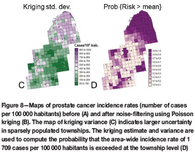
Figure 8A shows the map of prostate cancer incidence rates computed at the township level. The analysis was restricted to white males aged 65 years and over to minimize the impact of disparities in age distribution across the area and to attenuate the impact of variability in health coverage since all cases were covered by Medicare. In addition, 146 rates based on less than 10 cases were considered as unreliable and assigned a missing value. Even in townships with more than 10 cases rates can still be unstable, in particular in sparsely populated rural areas. This issue, known as the 'small number problem' in epidemiology, can be addressed geostatistically using a form of kriging with non-systematic measurement errors, called Poisson kriging (Goovaerts, 2009). The basic idea is to filter the noise attached to each rate using rates recorded in adjacent geographical units. Rates based on small population, hence less stable, receive less weight than rates recorded in densely populated areas in the kriging estimator. A major benefit of Poisson kriging over traditional statistical smoothers is that it allows the estimation of missing rates in addition to the filtering of noisy rates.

 

 

As for arsenic concentrations, this mapping technique requires the computation and modelling of a semivariogram. Two major differences are: (1) observations are rates and so are composed of a numerator (number of cancer cases) and a denominator (male population), and (2) the spatial supports of the observations are not points (area1 data) and are not uniform (townships have different sizes and shapes). The first problem is tackled by using a population-weighted semivariogram estimator to attenuate the impact of less stables rates in the modelling of the spatial variability. On the other hand, the spatial support of the data is accounted for using a form of block kriging, called area-to-area (ATA) kriging (Kyriakidis, 2004). The last issue is the fact that ATA kriging requires a point-support semivariogram model, whereas only a block-support semivariogram model is available since all observations are areal data. The derivation of a point-support semivariogram model from a block-support model is called deconvolution in geostatistics and is a well-known problem in the mining industry. Mining blocks tend, however, to be all squares of the same size, a situation very different from the administrative units that are manipulated in medical geography. A special iterative deconvolution procedure was recently developed for the case of irregular units (Goovaerts, 2008, 2011).

The map of noise-filtered rates (Figure 8B), called risks, displays much less variability than the original rate maps. In particular, some of the extreme incidence rates recorded in rural counties are no longer present. Higher incidences are observed in the northern area that is more rural (Figure 7) as well as in the cities of Detroit and Flint, which are less affluent than the college towns of Ann Arbor and Lansing. The map of the kriging variance (Figure 8C) looks similar to the map of population density (Figure 7) and reflects the greater reliability of rates estimated in densely populated areas compared to rates that were missing or estimated in rural areas. Following Goovaerts (2006), the probability distribution of the unknown risk can be modeled using a Gaussian distribution that has the Poisson kriging estimate and kriging variance as mean and variance. The probability of exceeding specific thresholds can thus be computed fairly easily and incorporates both the magnitude of the risk estimate and the associated uncertainty. For example, Figure 8D shows the probability that the area-wide incidence rate of 1709 cases per 100 000 habitants is exceeded.

 

Correlation analysis

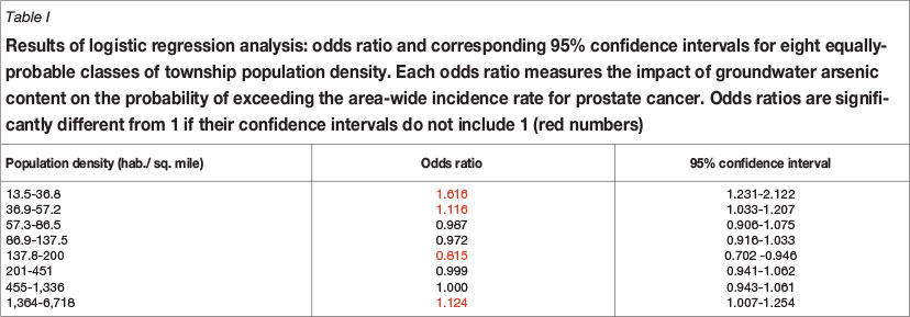
The relationship between the health outcome and putative covariates (arsenic level and population density) was analysed using logistic regression. The dependent variable is an indicator variable that takes a value of 1 if the probability of exceeding the area-wide incidence rate is above 0.5, and zero otherwise. The main predictor is the township-level concentration of arsenic displayed at the bottom of Figure 6. Given that rural townships are less likely to have access to regulated public water supply, one should expect the potential relationship between groundwater arsenic level and incidence of prostate cancer to be stronger where population density is low. This hypothesis was tested by using the following interaction term in the regression model: arsenic concentration × density class, where eight equally probable classes of population density (i.e. including similar number of townships) were created from Figure 7.

Regression results are reported in Table I. An odds ratio is a relative measure of association between an exposure (e.g. arsenic in groundwater) and an outcome (e.g. area-wide incidence rate for prostate cancer is exceeded with probability above 0.5). More precisely, the odds ratio represents the odds that the outcome will occur given a particular exposure, compared to the odds of the outcome occurring in the absence of that exposure. In the present case where the predictor is a continuous variable, the odds ratio can be interpreted as the change in odds if the arsenic concentration increases by 1 ppm. Table I shows that the risk for a township to exceed the area-wide incidence rate for prostate cancer increases significantly (odds ratio with 95% confidence interval larger than 1) for the first two classes of population density, that is in rural townships where habitants are more likely to rely on private wells for drinking water. The odds ratio is lower for all other classes that include townships that are more densely populated. The significant odds ratio recorded for the most urbanized townships is likely linked to the largest prevalence of chronic disease in neighborhoods of lower socio-economic status. A more detailed analysis is, however, warranted to tease out the impact of other contextual (e.g. poverty level, access to screening) and individual-level (e.g. smoking, groundwater consumption) covariates. Thus, the results of this analysis of aggregated data should be used mainly to design future case-control studies including cancer patients and healthy individuals with similar demographic characteristics.

 

Conclusions

The assessment of the health risk associated with environmental exposure has become the subject of considerable interest in our societies. This renew attention has led to the development of overlapping disciplines, such as geohealth; geoscience and public health; medical geology; epidemioe-cology; medical geography; medical ecology; clinical ecology; environmental medical epidemiology; geomedicine; geoepi-demiology; geology and health; geology, environment, and health; medical geography; and pathoecology, to name a few. All these fields of study are complex and require a multidisci-plinary approach that relies on a wide variety of specialists from geologists, geochemists, and medical doctors to biologists and veterinarians. A common thread is the recognition of the critical influence that place and location exert on the occurrence of health outcomes and environmental processes. To quote the Dutch philosopher Baruch Spinoza (1632-1677), 'Nothingin Nature is random.... A thing appears random only through the incompleteness of our knowledge.' Interactive mapping of epidemiological data with geographic and environmental features is a critical tool that facilitates the formulation of hypotheses and the identification of relationships regarding the spatial patterns of disease. Geostatistical methodology is likely to play a major role in this endeavour because of its ability to take into account the double aspect of randomness and spatial structure in the characterization of regionalized variables.

The application of geostatistics to the promising field of environmental epidemiology presents several methodological challenges that arise from the facts that: (1) data is very diverse and typically recorded over overlapping geographies (e.g. ZIP codes, census tracts), and (2) health outcomes are often aggregated over irregular spatial supports and consist of a numerator and a denominator (i.e. population size). Everyday geostatistical tools, such as semivariograms or kriging, thus cannot be implemented blindly. The last decade has witnessed the emergence of tools and techniques tailored to this new type of data. Irregular spatial supports can now be tackled thanks to area-to-area kriging and iterative deconvolution procedures. Similarly, Poisson and binomial kriging combined with population-weighted semivariogram estimators allow the incorporation of both the numerator and denominator in the processing of rate data. It is noteworthy that the general formulation of kriging introduced half a century ago could already accommodate different spatial supports for both the data and the predicted unit. The development of geographical information systems and dramatic increase in computational power finally made possible the implementation of these theoretical concepts.

The field of environmental health geostatistics is still in its infancy. Its growth cannot be sustained, or at least is meaningless, if it does not involve the end-users who are the epidemiologists, geologists, and GIS specialists working in health departments, geological surveys, and cancer registries. Critical components to its success include the publication of applied studies illustrating the merits of geostatistics over current empirical mapping methods, training through short courses, and updating of existing curricula, as well as the development of user-friendly software. The success of mining and environmental geostatistics, as we experience it today, can be traced back to its development outside the realm of spatial statistics, through the close collaboration of mathematically minded individuals and practitioners. Environmental health geostatistics will prove to be no different.

 

Acknowledgements

This research was funded by grant 1R21 ES021570-01A1 from the National Cancer Institute. The views stated in this publication are those of the author and do not necessarily represent the official views of the NCI.

 

References

Bowman, C., Bobrowski, P.T., and Selinus, O. 2003. Medical geology: New relevance in the earth sciences. Episodes, vol. 26, no. 4. pp. 270-278.

Cressie, N. 1993. Statistics for Spatial Data. Wiley, New York.         [ Links ]

Deutsch, C.V. and Journel, A.G. 1998. GSLIB: Geostatistical Software Library and User's Guide. 2nd edn. Oxford University Press, New York.         [ Links ]

Dissanayake, C.B. 2005. Essays on science and society: Global voices of science: Of stones and health: Medical geology in Sri Lanka. Science, vol. 309, no. 5736. pp. 883-885.         [ Links ]

Finkelman, R.B., Gingerich, H., Centeno, J.A., and Krieger, G. 2011. Medical geology issues in North America. Medical Geology: A Regional Synthesis. Selinus, O., Finkelman, R.B., and Centeno, J.A. (eds.). Springer, Dordrecht. pp. 1-27.         [ Links ]

Goovaerts, P. 1997. Geostatistics for Natural Resources Evaluation. Oxford University Press.         [ Links ]

Goovaerts, P. 1999. Geostatistics in soil science: state-of-the-art and perspectives. Geoderma, vol. 89, no. 1-2. pp. 1-45.         [ Links ]

Goovaerts, P. 2006. Geostatistical analysis of disease data: visualization and propagation of spatial uncertainty in cancer mortality risk using Poisson kriging and p-field simulation. International Journal of Health Geographics, vol. 5, no. 7.         [ Links ]

Goovaerts, P. 2007. Spatial uncertainty in medical geography: A geostatistical perspective. Encyclopedia of GIS. Shekhar, S. and Xiong, H. (eds.). Springer-Verlag, Berlin. pp. 1106-1112.         [ Links ]

Goovaerts, P. 2008. Kriging and semivariogram deconvolution in presence of irregular geographical units. Mathematical Geosciences, vol. 40, no. 1. pp. 101-128.         [ Links ]

Goovaerts, P. 2009. Medical geography: a promising field of application for geostatistics. Mathematical Geosciences, vol. 41, no. 3. pp. 243-264.         [ Links ]

Goovaerts, P. 2010. Combining areal and point data in geostatistical interpolation: Applications to soil science and medical geography. Mathematical Geosciences, vol. 42, no. 5. pp. 535-554.         [ Links ]

Goovaerts, P. 2011. A coherent geostatistical approach for combining choropleth map and field data in the spatial interpolation of soil properties. European Journal of Soil Sciences, vol. 62, no. 3. pp. 371-380.         [ Links ]

Goovaerts, P. 2012. Geostatistical analysis of health data with different levels of spatial aggregation. Spatial and Spatio-temporal Epidemiology, vol. 3, no. 1, pp. 83-92.         [ Links ]

Goovaerts, P., AvRuskin, G., Meliker, J., Slotnick, M., Jacquez, G.M., and Nriagu, J. 2005. Geostatistical modeling of the spatial variability of arsenic in groundwater of Southeast Michigan. Water Resources Research, vol. 41, no. 7. W07013 10.1029.         [ Links ]

Gotway, C.A., and Young, L.J. 2002. Combining incompatible spatial data. Journal of the American Statistical Association, vol. 97, no. 459. pp. 632-648.         [ Links ]

Gotway, C.A., and Young, L.J. 2007. A geostatistical approach to linking geographically-aggregated data from different sources. Journal of Computational and Graphical Statistics, vol. 16, no. 1. pp.115-135.         [ Links ]

Journel, A.G., and Huijbregts, C.J. 1978. Mining Geostatistics. Academic Press, New York.         [ Links ]

Krige, D.G. 1951. A statistical approach to some basic mine valuation problems on the Witwatersrand. Journal of the Chemical, Metallurgical and Mining Society of South AArica, vol. 52, no. 6. pp. 119-139.         [ Links ]

Kyriakidis, P. 2004. A geostatistical framework for area-to-point spatial interpolation. Geographical Analysis, vol. 36, no. 2. pp. 259-289.         [ Links ]

Kyriakidis, P. and Journel, A.G. 1999. Geostatistical space-time models. Mathematical Geology, vol. 31, no. 6. pp. 651-684.         [ Links ]

Lewis, D.R., Southwick, J.W., Ouellet-Hellstrom, R., Rench, J., and Calderon, R.L. 1999. Drinking water arsenic in Utah: A cohort mortality study. Environmental Health Perspectives, vol. 107, no. 5. pp. 359-365.         [ Links ]

May, J.M. 1950. Medical geography: its methods and objectives. Geographical Review, vol. 40. pp. 9-41.         [ Links ]

McLeod, K.S. 2000. Our sense of Snow: the myth of John Snow in medical geography. Social Science & Medicine, vol. 50, no. 7-8. pp. 923-935.         [ Links ]

Price, E.W. 1976. The association of endemic elephantiasis of the lower legs in East Africa with soil derived from volcanic rocks. Transactions of the Royal Society of Tropical Medicine and Hygiene, vol. 70, no. 4. pp. 288-295.         [ Links ]

Selinus, O. 2004. Medical geology: an emerging speciality. Terrae, vol. 1, no. 1. pp. 8-15.         [ Links ]

Selinus, O., Alloway, B.J., Centeno, J.A., Finkelman, R.B., Fuge, R., Lindh, U., and Smedley, P. eds. 2005. Essentials of Medical Geology - Impacts of the Natural Environment on Public Health. Elsevier Academic Press, Boston.         [ Links ]

Tobler, W. 1970. A computer movie simulating urban growth in the Detroit region. Economic Geography, vol. 46, no. 2. pp. 234-240.         [ Links ]

Waller, L.A., and Gotway, C.A. 2004. Applied Spatial Statistics for Public Health Data. John Wiley and Sons, New Jersey.         [ Links ]

Welch, A.H., Westjohn, D.B., Helsel, D.R., and Wanty, R.B. 2000. Arsenic in ground water of the United States: Occurrence and geochemistry. Ground Water, vol. 38, no. 4. pp. 589-604.         [ Links ]

Westjohn, D.B., Kölker, A., Cannon, W.F., and Sibley, D.F. 1998. Arsenic in ground water in the 'Thumb Area' of Michigan. The Mississippian Marshall Sandstone Revisited. Michigan: Its Geology and Geologic Resources, 5th Symposium. Michigan Department of Environmental Quality, East Lansing, Michigan. pp. 24-25.         [ Links ]